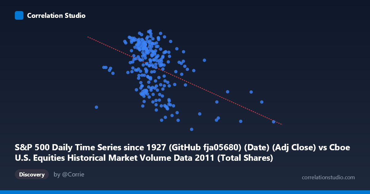
S&P 500 Daily Time Series since 1927 (GitHub fja05680) (Date) (Adj Close) vs Cboe U.S. Equities Historical Market Volume Data 2011 (Total Shares)

Pearson correlation (r): -0.4229
Spearman correlation: -0.3747
p-value: 0
Sample size (n): 252
95% confidence interval: -0.5194 to -0.3159
Granger causality: None
Granger optimal lag: 1
Time coverage: 2011-01-03 to 2011-12-30

AI analysis

Analysis: S&P 500 Adjusted Close vs. Total Shares Traded (2011)

Relationship Overview The scatterplot reveals a negative relationship between the S&P 500's adjusted closing price and total shares traded across U.S. equities exchanges in 2011. As the index price rises, trading volume in total shares tends to decline, and conversely, lower price levels are associated with higher share volumes. The linear regression equation (y = -2.15245E-07x + 1380.09) captures this downward slope, though the scatter around the regression line is considerable, indicating the relationship is real but far from deterministic. This pattern is consistent with well-documented market behavior: periods of stress and declining prices often generate elevated trading activity, while calmer, rising markets can see reduced participation.

Correlation Strength and Statistical Significance The Pearson correlation of r = -0.4229 indicates a moderate negative association. However, the r² of 0.1789 is the more sobering figure — it means that only ~17.9% of the variance in total shares traded is explained by the S&P 500 price level, leaving roughly 82% of the variance unexplained by this relationship alone. The 95% confidence interval of [-0.5194, -0.3159] is entirely negative, confirming the direction of the effect is reliable, and the p-value of 2.348E-12 makes this result highly statistically significant given n = 252 paired observations. That said, statistical significance here reflects that the effect is real and non-zero — not that it is large or practically dominant. The Granger causality results are notably absent: neither X→Y (F = 0.0032, p = 0.955) nor Y→X (F = 0.0014, p = 0.970) reaches significance at any conventional threshold, meaning that neither variable temporally predicts the other in a lead-lag sense. The correlation is contemporaneous rather than directional — knowing yesterday's price does not help predict today's volume, and vice versa.

Notable Patterns, Clusters, and Outliers Several features stand out in the data. There is a visible cluster of high-volume observations at lower price ranges (roughly X < 500M), which likely corresponds to the market stress periods of summer/fall 2011 — when the U.S. debt ceiling crisis, S&P sovereign downgrade, and European debt contagion fears drove both lower prices and elevated trading. Conversely, points with higher price values (X 700M) tend to congregate at lower share volumes, consistent with the calmer early-year period. A handful of apparent outliers are visible at extreme X values (approaching ~878M and ~1.2B range) with relatively modest Y values, suggesting days of very high notional or price-weighted volume that did not translate proportionally into share counts — possibly reflecting index composition or large-cap dominance effects. The relationship also appears heteroscedastic, with greater Y-variance at lower price levels than at higher ones, hinting that a simple linear model may not be the optimal fit.

Confounding Factors and Caveats Several important caveats apply. First, 2011 was an atypical year with multiple macro shocks (debt ceiling, eurozone crisis, flash crash aftershocks), making the volume-price dynamic potentially unrepresentative of other periods. Second, the axis labels appear swapped in the dataset metadata — the X-axis is described as originating from the Cboe volume dataset while the Y-axis is sourced from the S&P 500 price dataset, which warrants verification before drawing firm conclusions. Third, the negative correlation may be partly driven by a shared time trend: prices trended lower mid-year while volumes spiked, creating a spurious or inflated association when observations are treated as independent cross-sectional points rather than a time series. Fourth, total shares traded is sensitive to stock splits, index rebalancing, and the growth of high-frequency trading, all of which can decouple share counts from meaningful economic activity. The lack of Granger causality strongly suggests these variables move together due to common external drivers rather than any direct causal mechanism.

Actionable Insights and Further Investigation Given that only ~18% of variance is explained and no temporal predictive relationship exists, practitioners should avoid using price level alone as a volume forecasting signal. More productive next steps would include: (1) decomposing the time series into trend and volatility components (e.g., using VIX as a covariate) to test whether volatility — not price level — is the true driver of elevated share volume; (2) segmenting the data by market regime (stress vs. calm periods) to test whether the correlation strengthens meaningfully during drawdowns; (3) examining notional value and trade counts from the same Cboe dataset alongside total shares to disentangle the effects of price-per-share from trading intensity; and (4) extending the analysis beyond 2011 to test whether this negative relationship is structurally stable or an artifact of that year's specific volatility environment. A non-linear or quantile regression approach may also better capture the apparent heteroscedasticity observed at lower price levels.

X dataset: Cboe U.S. Equities Historical Market Volume Data 2011

Y dataset: S&P 500 Daily Time Series since 1927 (GitHub fja05680) (Date)

Part of experiment: Daily - Cboe U.S. Equities Historical Market Volume Data 2011 vs S&P 500 Daily Time Series since 1927 (GitHub fja05680) (Date)