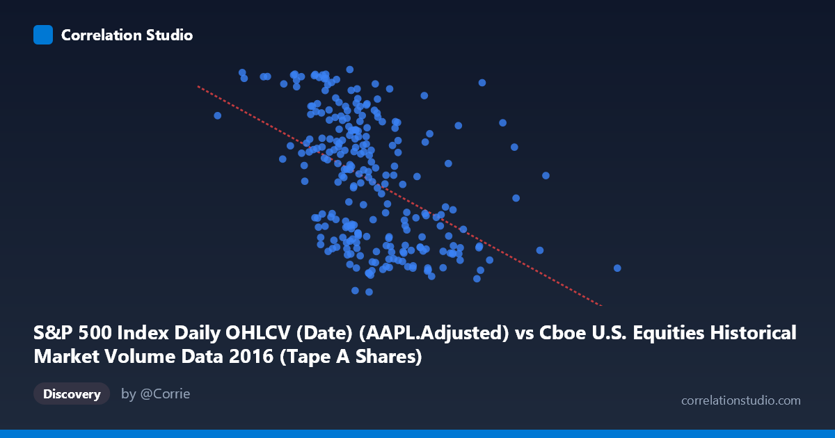
S&P 500 Index Daily OHLCV (Date) (AAPL.Adjusted) vs Cboe U.S. Equities Historical Market Volume Data 2016 (Tape A Shares)
- Pearson correlation (r)
- -0.4626
- Spearman correlation
- -0.4963
- p-value
- 0
- Sample size (n)
- 252
- 95% confidence interval
- -0.5545 to -0.3596
- Granger causality
- None
- Granger optimal lag
- 1
AI analysis
Scatterplot Analysis: AAPL Adjusted Price vs. Cboe Tape A Share Volume (2016)
1. Relationship Overview The visualization reveals a negative relationship between Apple's adjusted stock price (X-axis) and Cboe U.S. Equities Tape A share volume (Y-axis) across 252 trading days in 2016. As AAPL's adjusted price increases, Tape A share volume tends to decline, and vice versa. The linear regression equation (y = -6.29E-08x + 120.296) confirms this inverse slope, meaning that for every ~$16 increase in AAPL's price, Tape A volume is predicted to decrease by approximately one unit. Visually, the cloud of points likely shows a downward-sloping trend, though with considerable scatter, suggesting the relationship is real but far from deterministic.
2. Correlation Strength, Direction, and Causality The Pearson correlation of r = -0.4626 indicates a moderate negative correlation — meaningful but not strong. Crucially, the R² of 0.2140 means that AAPL's price explains only about 21.4% of the variance in Tape A volume, leaving nearly 79% of the variation unexplained by this relationship alone. The 95% confidence interval of [-0.5545, -0.3596] is entirely negative, confirming the direction is robustly inverse, and the p-value of 9.1×10⁻¹⁵ establishes overwhelming statistical significance — this is not a chance association given n=252. However, statistical significance must not be conflated with practical or causal significance. The Granger causality tests failed in both directions (X→Y: F=0.18, p=0.67; Y→X: F=2.21, p=0.14), meaning neither variable temporally predicts the other with a one-period lag. This is a critical finding: despite the correlation, there is no evidence of directional temporal predictability between these two series.
3. Notable Patterns and Outliers Several features likely stand out in the scatter cloud. The data points cluster most densely in the AAPL price range of roughly $220–$320M adjusted (reflecting the X mean of ~$272M), with Tape A volume scattered broadly between ~89 and 117. A few potential outliers are visible in the sample — notably the point near (190M, 116.55) and (176M, 105.82), which represent lower AAPL prices but divergent volume readings, and points like (271M, 89.01) sitting well below the trend line. The spread appears heteroscedastic, with greater Y variance at lower X values, suggesting the negative relationship may not be uniform across the price range. There is no strong evidence of a clean linear fit; the wide scatter implies possible non-linear or regime-dependent behavior that a simple linear model fails to capture.
4. Confounding Factors and Caveats Several important caveats apply. First, this correlation likely reflects a shared temporal dynamic rather than a direct mechanistic link: both AAPL's price trajectory and overall market volume in 2016 were driven by macro events (Fed policy, Brexit, U.S. election), creating spurious co-movement. Second, the axis labels appear transposed relative to what might be intuitive — Tape A volume is on the Y-axis but belongs to the S&P 500 dataset, while AAPL adjusted price is on the X-axis from the Cboe dataset, which is an unusual pairing that warrants data provenance review. Third, AAPL price is a single-stock metric being compared against a broad market volume measure, making any causal story implausible without controlling for overall market capitalization changes, index composition shifts, or electronic trading trends throughout 2016. Seasonality and event-driven volume spikes (earnings, option expiration dates) are uncontrolled confounders.
5. Actionable Insights and Further Investigation Given the moderate but unexplained correlation and absence of Granger causality, no trading or operational strategy should be built on this relationship alone. Recommended next steps include: (a) decomposing the time series to test whether the correlation persists after removing shared trend components (e.g., cointegration testing or first-differencing); (b) extending the Granger causality analysis to longer lag structures (2–10 periods) since a one-period lag may be insufficient to capture volume-price dynamics; (c) controlling for VIX or market-wide volatility as a likely common driver of both series; and (d) replicating the analysis across multiple years to assess whether this 2016 relationship is stable or an artifact of that year's specific market regime. The ~79% unexplained variance is the most actionable signal here — it strongly motivates a multivariate modeling approach rather than relying on this bivariate relationship.
X dataset: Cboe U.S. Equities Historical Market Volume Data 2016
Y dataset: S&P 500 Index Daily OHLCV (Date)
Part of experiment: Daily - Cboe U.S. Equities Historical Market Volume Data 2016 vs S&P 500 Index Daily OHLCV (Date)