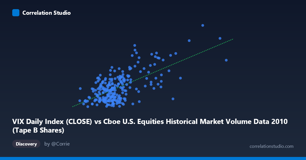
VIX Daily Index (CLOSE) vs Cboe U.S. Equities Historical Market Volume Data 2010 (Tape B Shares)

Pearson correlation (r): 0.6474
Spearman correlation: 0.4745
p-value: 0
Sample size (n): 252
95% confidence interval: 0.5694 to 0.7139
Granger causality: Y → X
Granger optimal lag: 1

AI analysis

Scatterplot Analysis: VIX vs. Tape B Share Volume (2010)

Relationship Overview

The scatterplot reveals a moderately strong positive relationship between the CBOE Volatility Index (VIX) daily close values and Tape B share volumes in U.S. equity markets during 2010. As VIX levels rise — reflecting greater implied market uncertainty — Tape B trading volumes tend to increase in tandem. This is broadly consistent with well-established market microstructure theory: heightened fear or uncertainty drives investors to reposition portfolios, generating elevated transaction activity across equity exchanges. The linear regression equation (y = 7.92×10⁻⁸x + 13.60) captures this upward trend, though the scatter around the regression line suggests that the relationship is real but far from deterministic.

Correlation Strength and Statistical Significance

The Pearson correlation of r = 0.6474 indicates a moderate-to-strong positive association, but the more informative metric is r² = 0.4192: VIX levels explain approximately 42% of the variance in Tape B share volume, leaving 58% attributable to other factors. The 95% confidence interval [0.5694, 0.7139] is reasonably tight and lies entirely above zero, and the p-value is effectively zero across a paired sample of 252 observations drawn from a population of 3,302 — making the result highly statistically robust with negligible risk of a false positive. Crucially, the Granger causality test identifies a unidirectional temporal relationship: Y Granger-causes X (F = 7.99, p = 0.005) at a one-period lag, while X→Y falls short of significance (F = 3.60, p = 0.059). In practical terms, this suggests that past VIX levels are a meaningful predictor of future Tape B volume, but the reverse does not hold statistically — volume changes do not reliably precede VIX movements in this dataset.

Notable Patterns, Clusters, and Outliers

The data display a clear clustering of observations in the lower-left quadrant — VIX values roughly between 15–25 paired with lower share volumes — reflecting the relatively calm, range-bound equity environment that characterized much of 2010's mid-year period. Above VIX ≈ 30, the scatter widens considerably, indicating heteroscedasticity: at elevated fear levels, volume responses become more variable and less predictable. Several notable outliers appear in the upper-right region (e.g., points near VIX ~41 and volume ~316 million), likely corresponding to specific stress episodes such as the May 2010 Flash Crash or European sovereign debt concerns. These high-leverage points may be exerting disproportionate influence on the regression slope and inflating the overall r value.

Confounding Factors and Interpretive Caveats

Several important caveats apply. First, Tape B specifically covers NYSE American (AMEX) and regional exchange listings — a subset of total market activity — so findings may not generalize to broader volume metrics. Second, both variables are time-series with known autocorrelation, which can artificially inflate correlation coefficients if not properly accounted for; the Granger framework partially addresses this, but spurious co-movement driven by shared macroeconomic shocks (e.g., Fed announcements, earnings seasons) cannot be ruled out. Third, the heteroscedasticity observed at high VIX levels suggests a linear model may be misspecified — a log-log or piecewise regression might better capture the true functional form. Finally, 2010 was an atypical year bookended by post-crisis recovery dynamics and specific volatility events, limiting the generalizability of these findings to other market regimes.

Actionable Insights and Further Investigation

Practitioners could explore using VIX as a one-period-lagged predictor of Tape B volume in short-term trading or liquidity management models, given the statistically significant Granger causality result. However, given that 58% of variance remains unexplained, this should be supplemented with additional predictors — such as overall market returns, options open interest, or macroeconomic surprise indices. Methodologically, it would be valuable to: (1) re-estimate the model in log space to address heteroscedasticity; (2) test for structural breaks around the Flash Crash (May 6, 2010) to assess whether one regime is driving the bulk of the correlation; and (3) extend the analysis across multiple years to determine whether the VIX→Tape B volume relationship is stable or period-specific. A rolling-window correlation analysis would reveal whether this predictive relationship strengthens during crisis periods and attenuates during calm markets.

X dataset: Cboe U.S. Equities Historical Market Volume Data 2010

Y dataset: VIX Daily Index

Part of experiment: Daily - Cboe U.S. Equities Historical Market Volume Data 2010 vs VIX Daily Index