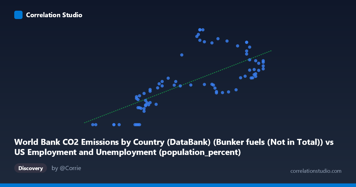
World Bank CO2 Emissions by Country (DataBank) (Bunker fuels (Not in Total)) vs US Employment and Unemployment (population_percent)
- Pearson correlation (r)
- 0.7072
- Spearman correlation
- 0.7554
- p-value
- 0
- Sample size (n)
- 80
- 95% confidence interval
- 0.5772 to 0.8023
- Granger causality
- Y → X
- Granger optimal lag
- 10
AI analysis
Scatterplot Analysis: Bunker Fuel CO₂ Emissions vs. US Employment Population Percent
1. Overall Relationship The scatterplot reveals a moderate-to-strong positive relationship between World Bank bunker fuel CO₂ emissions and US employment as a percentage of population, spanning eight decades from 1941 to 2020. As bunker fuel emissions rise (roughly 56–67 units on the x-axis), US employment rates tend to increase as well, following a broadly upward linear trend captured by the regression equation y = 97.52x − 5356.05. However, the scatter around this line is substantial, and the data exhibit notable clustering and heteroscedasticity — particularly a wide spread of Y values in the mid-to-upper X range — suggesting the linear model, while informative, is an incomplete description of the relationship.
2. Correlation Strength, Direction, and Causality The Pearson correlation of r = 0.707 indicates a moderately strong positive association, but the more telling statistic is r² = 0.50: exactly half the variance in US employment rates is explained by bunker fuel emissions, meaning the other half is driven by factors entirely outside this model. The 95% confidence interval [0.577, 0.802] is reasonably tight and does not approach zero, and the p-value of 2.25 × 10⁻¹³ confirms the relationship is overwhelmingly unlikely to be a chance artifact given n = 80 paired observations. Critically, the Granger causality analysis reverses the intuitive causal arrow: Y Granger-causes X (F = 2.05, p = 0.048) with a 10-period lag, meaning past US employment rates have statistically significant predictive power over future bunker fuel emissions — but not vice versa (X→Y: p = 0.155). This suggests that economic activity and labor market conditions may precede and help drive shipping/aviation fuel demand, rather than emissions driving employment.
3. Notable Patterns, Clusters, and Outliers Several structural features stand out. First, there is a distinct cluster of zero-valued Y observations (employment % = 0.00) spanning lower X values (~55.8–58.9), likely corresponding to early wartime or data-gap years where employment figures were unavailable or definitionally different. These zero values distort the regression and should be treated as missing data rather than true zero employment. Second, in the X range of roughly 62–64, there is a striking bimodal vertical spread — some observations cluster near 550–700 while others shoot above 1,370–1,590 — suggesting two distinct behavioral regimes at similar emission levels, possibly reflecting pre- and post-economic-shock periods (e.g., recessions, COVID-19). Third, the upper-right cluster (X 65, Y 800) shows tighter, more consistent co-movement, potentially representing the more globalized post-1990 era.
4. Confounding Factors and Caveats This correlation almost certainly reflects a common driver rather than a direct mechanism: long-run global economic growth simultaneously expands labor markets and increases demand for international shipping and aviation fuel. The dataset pairing itself is conceptually unusual — US domestic employment rates from BLS data are being correlated with global bunker fuel emissions tracked by the World Bank, spanning entirely different geographic and sectoral scopes. Structural breaks from events like World War II mobilization, the 1970s oil shocks, the 2008 financial crisis, and the 2020 COVID-19 pandemic likely create non-stationary regime shifts that violate the assumptions of a single linear model. The 10-period Granger lag also warrants caution: with annual data, a 10-year lag is unusually long and may be capturing a spurious low-frequency trend rather than a genuine predictive mechanism. The zero-valued Y entries further compromise regression validity if left untreated.
5. Actionable Insights and Further Investigation The Granger causality finding — that employment predicts emissions with a decade-long lag — is the most scientifically interesting result here and merits deeper investigation. Analysts should decompose both series (e.g., via HP filter or first-differencing) to remove shared secular trends before re-examining the correlation, as much of the r = 0.707 may be trend-on-trend cointegration rather than a meaningful cyclical relationship. It would be valuable to test whether US employment specifically drives US-originated bunker fuel demand (domestic shipping/aviation), which would make the causal story more mechanistically coherent. Additionally, excluding or imputing the zero-Y records and testing a piecewise or non-linear model for the evident mid-range bifurcation could substantially improve model fit beyond the current 50% explained variance. Finally, introducing GDP, oil prices, or trade volume as control variables in a multivariate framework would help isolate whether any independent relationship between employment and bunker emissions survives after accounting for the dominant confound of aggregate economic growth.
X dataset: US Employment and Unemployment
Y dataset: World Bank CO2 Emissions by Country (DataBank)
Part of experiment: Yearly - US Employment and Unemployment vs World Bank CO2 Emissions by Country (DataBank)