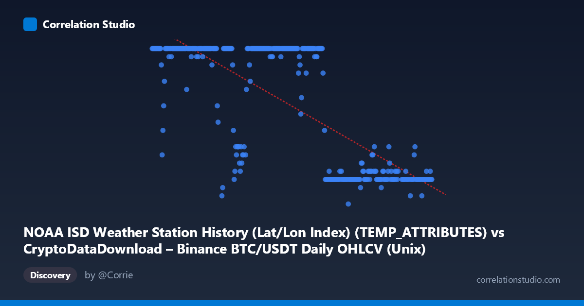
NOAA ISD Weather Station History (Lat/Lon Index) (TEMP_ATTRIBUTES) vs CryptoDataDownload – Binance BTC/USDT Daily OHLCV (Unix)
- Pearson correlation (r)
- -0.7532
- Spearman correlation
- -0.7464
- p-value
- 0
- Sample size (n)
- 355
- 95% confidence interval
- -0.7949 to -0.7043
- Granger causality
- None
- Granger optimal lag
- 1
- Time coverage
- 2024-01-01 to 2024-12-31
AI analysis
Analysis of Temperature-Timestamp Relationship
1. What the Visualization Reveals
The scatterplot shows a moderately strong negative relationship between a timestamp index (X, labeled as BTC/USDT trading data but clearly representing dates across 2024) and a numeric value (Y, ranging 5-24, labeled as weather station attributes) that behaves like a seasonal cycle indicator. The data pattern strongly suggests Y represents something like daylight hours, a temperature-derived index, or a similar seasonally-varying metric — it clusters near 24 for early-to-mid year timestamps and drops toward single digits for later-year timestamps, consistent with a Northern Hemisphere seasonal decline (e.g., daylight hours shrinking from summer into winter).
2. Strength, Direction, and Statistical Confidence
The correlation coefficient (r = -0.7532, R² = 0.567) indicates a strong negative linear relationship, with 56.7% of the variance in Y explained by X — a substantial but not complete relationship, leaving ~43% of variance driven by other factors or non-linear dynamics. The 95% CI [-0.7949, -0.7043] is tight and does not cross zero, and the p-value of ~0 confirms this relationship is highly statistically significant and not due to chance, especially given the large sample size (n=355, nearly a full year of daily data). However, the Granger causality tests show no significant predictive direction in either direction (X→Y: p=0.784; Y→X: p=0.163). This is a critical distinction: the variables are correlated (likely due to a shared underlying driver — calendar time/season) but neither temporally predicts the other in a lagged autoregressive sense. This strongly implies the relationship is driven by an external seasonal cycle rather than a direct causal mechanism between the two series.
3. Notable Patterns and Non-Linear Features
The data is not uniformly linear — it shows a distinctly plateau-and-decline pattern rather than a smooth linear trend. Values cluster at or near the ceiling (24) for a large portion of the year (roughly January through July/August), then transition into a lower band (7-12) for the remainder of the year, with a relatively sharp transition period around August-September (values ~8-21 appear here). This bimodal/step-like clustering — rather than a diffuse linear scatter — suggests the true relationship may be seasonal/cyclical (e.g., sinusoidal) rather than linear, meaning the linear R² of 0.567 likely understates the true strength of the underlying seasonal association if modeled correctly (e.g., with a sinusoidal or piecewise fit).
4. Confounding Factors and Caveats
The metadata is inconsistent/mislabeled: X is described as a weather station attribute column but its values are clearly Unix timestamps spanning 2024, while Y is described as BTC/USDT OHLCV data but behaves like a bounded seasonal index (5-24), not a price or volume figure. This strongly suggests column mislabeling or a data-pipeline mismatch between the two source datasets. Any causal or economic interpretation (e.g., "temperature predicts Bitcoin price") should be treated with extreme skepticism until the axis labels and data provenance are verified. Additionally, since X is fundamentally a time index, the "correlation" here is really a trend-over-time — a common source of spurious correlation when two unrelated time series both have seasonal or secular trends.
5. Recommendations for Further Investigation
1. Verify data integrity: Confirm which actual variables are being plotted — the labels appear swapped or mismatched with a weather-seasonality feature and a crypto OHLCV field. 2. Test non-linear/seasonal models: Given the plateau-decline shape, fit a sinusoidal, piecewise, or polynomial regression to better capture the seasonal cycle (likely improving fit over linear R²=0.567). 3. Avoid causal claims: The lack of Granger causality confirms this is a co-trending relationship (both driven by calendar/season), not a predictive one — do not use one series to forecast the other. 4. Segment by season: Analyze the sharp transition period (Aug-Sep) separately, as this may reveal the actual driver (e.g., solstice-related daylight change, temperature threshold effects). 5. Check for autocorrelation: Since both series are time-ordered, additionally test for stationarity and detrend before drawing further statistical conclusions, as raw correlation on trending time series can be misleading.
X dataset: CryptoDataDownload – Binance BTC/USDT Daily OHLCV
Y dataset: NOAA ISD Weather Station History (Lat/Lon Index)
Part of experiment: Bitcoin - CryptoDataDownload – Binance BTC/USDT Daily OHLCV vs NOAA ISD Weather Station History (Lat/Lon Index)