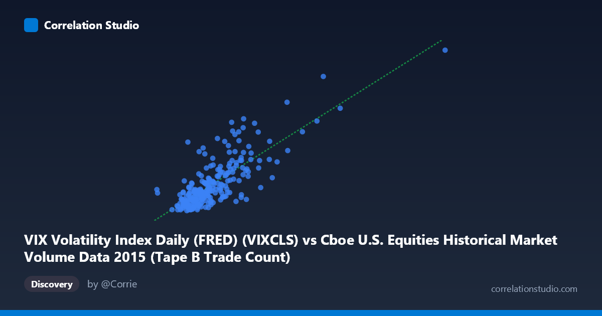
VIX Volatility Index Daily (FRED) (VIXCLS) vs Cboe U.S. Equities Historical Market Volume Data 2015 (Tape B Trade Count)
- Pearson correlation (r)
- 0.7902
- Spearman correlation
- 0.7286
- p-value
- 0
- Sample size (n)
- 252
- 95% confidence interval
- 0.7387 to 0.8325
- Granger causality
- None
- Granger optimal lag
- 1
AI analysis
Scatterplot Analysis: VIX Volatility Index vs. Tape B Trade Count (2015)
Relationship Overview
The scatterplot reveals a clear positive relationship between the CBOE VIX Volatility Index and Tape B trade count on U.S. equities exchanges throughout 2015. As implied volatility rises — reflecting heightened market fear or uncertainty — the number of trades executed on Tape B venues increases correspondingly. This is economically intuitive: periods of elevated volatility typically drive higher trading activity as market participants react to uncertainty by repositioning, hedging, or speculating. The linear regression equation (y = 3.67×10⁻⁵x + 5.678) confirms a positive slope, suggesting that each unit increase in VIX associates with a meaningful upward shift in trade count.
Correlation Strength and Statistical Significance
The correlation is strong at r = 0.790, and the r² of 0.624 indicates that approximately 62.4% of the variance in Tape B trade count is explained by VIX levels — a notably high figure for financial market data. The 95% confidence interval [0.739, 0.833] is relatively tight and does not approach zero, reinforcing the robustness of this finding. The p-value of effectively 0 across n = 252 paired observations drawn from a population of N = 3,302 confirms this is not a chance association. However, despite this strong contemporaneous correlation, Granger causality tests find no significant predictive temporal direction in either direction (X→Y: F = 0.483, p = 0.488; Y→X: F = 0.0004, p = 0.983). This is a critical caveat: VIX and Tape B trade count move together, but neither reliably predicts the other at a one-period lag. They likely share common drivers rather than one causing the other.
Patterns, Clusters, and Outliers
The data exhibits a clear lower-left cluster dominating the distribution — most observations fall in the VIX range of roughly 130,000–350,000 (trade count) with VIX values between 11 and 20, reflecting the calmer, low-volatility environment that characterized much of early-to-mid 2015. Above VIX ≈ 22–24, the scatter becomes notably sparser and more dispersed, consistent with episodic volatility spikes. Several high-leverage outliers are visible in the upper-right region — for example, the points near (640,679; 36.02) and (621,009; 28.03) — which correspond to extreme market stress events, likely the August 2015 flash crash or the late-summer China-driven equity selloff. These outliers appear to exert considerable influence on the regression line and correlation coefficient, and their removal would likely weaken r substantially.
Confounding Factors and Caveats
Several important caveats apply. First, reverse causality and simultaneity are plausible: high trade volumes could themselves amplify intraday price swings, which feed back into VIX — the Granger null result supports this bidirectional ambiguity rather than a clean causal story. Second, both variables are likely driven by common macro shocks (e.g., Fed policy announcements, geopolitical events, earnings seasons), making this a classic case of spurious correlation driven by latent confounders. Third, the outlier sensitivity is significant — 2015 contained the August volatility event, and a handful of extreme days may be disproportionately inflating r². Fourth, Tape B specifically captures regional exchange and dark pool activity, which may respond differently to volatility than Tape A or C venues, limiting generalizability. Finally, the relationship is modeled as linear, but the fan-shaped spread at higher VIX values hints at heteroscedasticity, suggesting a log-log or power-law specification might be more appropriate.
Actionable Insights and Further Investigation
Practitioners could explore using VIX as a real-time liquidity signal for Tape B venues, since the strong contemporaneous correlation suggests monitoring VIX thresholds (e.g., VIX 20 or 25) could anticipate elevated trade volumes and associated market impact costs. For researchers, several follow-up analyses are warranted: (1) re-run the analysis excluding the August 2015 volatility episode to assess whether the correlation is structurally stable or outlier-driven; (2) apply a log transformation to both variables to address heteroscedasticity and test whether explanatory power improves; (3) extend to multi-year data to confirm whether 2015 is representative or anomalous; (4) decompose by market regime (VIX < 15, 15–20, 20) to test for threshold effects; and (5) include additional predictors such as S&P 500 returns, bid-ask spreads, or macroeconomic releases to better isolate VIX's marginal contribution beyond shared systemic shocks.
X dataset: Cboe U.S. Equities Historical Market Volume Data 2015
Y dataset: VIX Volatility Index Daily (FRED)
Part of experiment: Daily - Cboe U.S. Equities Historical Market Volume Data 2015 vs VIX Volatility Index Daily (FRED)