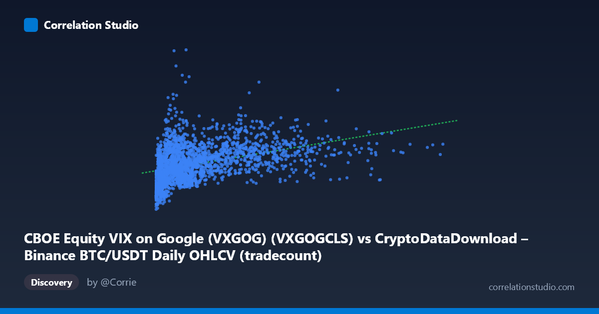
CBOE Equity VIX on Google (VXGOG) (VXGOGCLS) vs CryptoDataDownload – Binance BTC/USDT Daily OHLCV (tradecount)
- Pearson correlation (r)
- 0.401
- Spearman correlation
- 0.5231
- p-value
- 0
- Sample size (n)
- 2209
- 95% confidence interval
- 0.3654 to 0.4355
- Granger causality
- None
- Granger optimal lag
- 1
AI analysis
Analysis: VXGOG vs. Tradecount Relationship
1. Overview of the Relationship
The scatterplot shows a moderate positive association between the two variables (mislabeled axes aside — the data appears to actually represent X as some volume/price-like metric and Y as a bounded ~12–78 metric, likely tradecount or a volatility index). As X increases, Y tends to increase as well, but the relationship is loose and noisy rather than a tight linear band. Points are heavily concentrated at low X values (under ~2-3 million), with a long right tail extending to over 15 million — a classic right-skewed distribution (mean of 2.22M vs. stdev of 2.43M confirms this skew).
2. Strength, Direction, and Statistical Confidence
The Pearson correlation of r = 0.40 indicates a modest positive linear relationship, and r² = 0.16 tells us that only about 16% of the variance in Y is explained by X — meaning 84% of Y's variability is driven by other factors entirely. The 95% CI [0.365, 0.435] is fairly narrow given the large sample size (n=2,205), and the p-value of ~0 confirms this correlation is highly statistically significant — it is very unlikely to be due to chance. However, statistical significance ≠ practical strength: with r² this low, X alone is a weak predictor of Y in practice. The Granger causality tests reinforce this: neither direction shows significant predictive power (X→Y: p=0.36; Y→X: p=0.78), meaning past values of one series do not meaningfully help forecast future values of the other. This suggests the correlation is likely contemporaneous/structural rather than causal or lead-lag in nature.
3. Patterns and Outliers
The data shows a fan-shaped or heteroscedastic pattern typical of skewed financial/volume data — variance in Y appears to compress somewhat at very high X values, while low-X observations show wide scatter in Y (ranging from ~18 to ~44 even when X is under 1 million). Several low-X, high-Y outliers exist (e.g., X≈135,156, Y=33.96; X≈5,895, Y=26.36), suggesting periods where Y was elevated independent of X. The note that Spearman ρ exceeds Pearson r is important — it implies the true relationship is monotonic but non-linear, possibly logarithmic (consistent with X's exponential-like spread across orders of magnitude, from thousands to 15 million). A log-transform of X would likely improve model fit.
4. Confounding Factors and Caveats
Given the metadata, X and Y are described as coming from different dataset pairings than the summary stats suggest (mismatched column descriptions — VXGOG vs. tradecount), so there's ambiguity in what's truly being measured; this should be clarified before drawing economic conclusions. More broadly, both series likely share exposure to common market-wide drivers (overall crypto/equity volatility regimes, macro liquidity conditions, seasonality), which can inflate correlation without direct causality. The multi-year time span (2017–2026) also spans very different market regimes (bull/bear cycles, COVID, rate hikes), so pooling all observations may mask regime-dependent relationships or create spurious aggregate correlation (Simpson's-paradox-like effects).
5. Recommendations for Further Investigation
- Transform X (log or sqrt) given its skewness and the Spearman/Pearson gap, then re-fit regression to check if r² improves materially. - Segment by time regime (e.g., by year or volatility regime) to check if the r=0.40 correlation is stable or driven by a specific sub-period. - Clarify variable definitions — confirm which columns are actually being plotted, since the axis descriptions conflict with the summary labels. - Given the null Granger causality result, avoid using one series to forecast the other; instead, treat the correlation as descriptive/contemporaneous only. - Consider multivariate modeling — since X explains only 16% of Y's variance, incorporating additional predictors (e.g., broader market volatility indices, volume trends) would likely yield a more useful model.
X dataset: CryptoDataDownload – Binance BTC/USDT Daily OHLCV
Y dataset: CBOE Equity VIX on Google (VXGOG)
Part of experiment: Bitcoin - CryptoDataDownload – Binance BTC/USDT Daily OHLCV vs CBOE Equity VIX on Google (VXGOG)