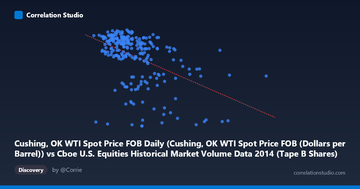
Cushing, OK WTI Spot Price FOB Daily (Cushing, OK WTI Spot Price FOB (Dollars per Barrel)) vs Cboe U.S. Equities Historical Market Volume Data 2014 (Tape B Shares)
- Pearson correlation (r)
- -0.4731
- Spearman correlation
- -0.4779
- p-value
- 0
- Sample size (n)
- 252
- 95% confidence interval
- -0.5637 to -0.3712
- Granger causality
- None
- Granger optimal lag
- 2
AI analysis
Analysis: WTI Crude Oil Price vs. Cboe Tape B Share Volume (2014)
Relationship Overview
The scatterplot reveals a negative relationship between WTI crude oil spot prices (X-axis) and Cboe Tape B equity share volume (Y-axis) across 252 trading days in 2014. As oil prices increase, Tape B share volume tends to decrease, and vice versa. The linear regression equation (y = -2.70×10⁻⁷x + 113.514) confirms this inverse slope, suggesting that for every ~$3.70 increase in oil price per barrel, Tape B volume declines by roughly one unit. Visually, the data forms a loosely dispersed cloud with a downward trend, but substantial scatter is immediately apparent, indicating that the relationship is real but far from deterministic.
Correlation Strength and Statistical Significance
The correlation coefficient of r = -0.4731 indicates a moderate negative association, but the explained variance tells the more important story: r² = 0.2238 means only ~22.4% of the variance in Tape B volume is accounted for by oil price movements, leaving approximately 77.6% attributable to other factors. The 95% confidence interval of [-0.5637, -0.3712] is entirely negative and relatively tight, providing strong assurance that the true population correlation is genuinely inverse rather than a sampling artifact. The p-value of 1.776×10⁻¹⁵ is extraordinarily small against a population of N = 3,686, making this correlation highly statistically significant. However, the Granger causality results are notably inconclusive: neither direction (X→Y: F = 1.80, p = 0.168; Y→X: F = 0.295, p = 0.745) reaches significance at the optimal 2-period lag. This means that while oil prices and Tape B volume are contemporaneously correlated, neither variable reliably predicts future movements in the other — a critical distinction between correlation and temporal causation.
Notable Patterns, Clusters, and Outliers
Several structural features stand out in the data. There appears to be a distinct lower cluster of points with very low Tape B values (~53–67 range) scattered across the oil price spectrum, particularly visible at points like (155.9M, 55.97), (100.7M, 55.25), (50.96M, 54.59), and (73.34M, 54.14). These low-volume outliers suggest discrete low-volume trading days — likely holidays, half-sessions, or unusual market closures — that are structurally different from typical trading days and could be heavily distorting the correlation. The bulk of the data, by contrast, clusters between oil prices of $55–$105/barrel and Tape B volumes of 85–110, forming a more coherent but still diffuse negative relationship. The high-oil-price region (above $140M+ on X) shows notably lower volume values, reinforcing the downward trend at extremes.
Confounding Factors and Caveats
Several important caveats limit causal interpretation. First, 2014 was a structurally unique year for oil markets, featuring a dramatic price collapse in the second half from ~$100/barrel to below $60, while equity markets simultaneously experienced volatility shifts — these macro regime changes could create a spurious correlation driven by shared time trends rather than a true functional relationship. Second, Tape B specifically covers NYSE American (AMEX)-listed securities, many of which include energy-sector ETFs and smaller energy companies; a shared sensitivity to the energy sector could create mechanical correlation without direct causation. Third, the low-volume day outliers identified above, if not removed or treated separately, artificially inflate the apparent correlation strength. Finally, broader macroeconomic variables — Federal Reserve policy, USD strength, risk-off sentiment — likely drive both oil prices and equity volumes simultaneously, making this a classic case of potential common-cause confounding.
Actionable Insights and Further Investigation
Given the moderate but unexplained variance and the absence of Granger causality, practitioners should avoid using oil prices as a direct predictive signal for Tape B volume in trading or liquidity models. Instead, the following investigative steps are warranted: (1) Remove or flag structural low-volume days (holidays/half-sessions) and re-run the correlation to assess whether the relationship persists or weakens substantially. (2) Decompose the time series into pre- and post-oil-crash periods (roughly June 2014 as a breakpoint) to test whether the correlation is regime-dependent. (3) Investigate whether energy-sector-heavy Tape B constituents are driving the relationship by isolating volume by sector or security type. (4) Include multivariate controls — USD index, VIX, S&P 500 returns — to partial out shared macro drivers and isolate any residual oil-volume relationship. The true signal here may be more nuanced and sector-specific than a simple bivariate correlation can reveal.
X dataset: Cboe U.S. Equities Historical Market Volume Data 2014
Y dataset: Cushing, OK WTI Spot Price FOB Daily
Part of experiment: Daily - Cboe U.S. Equities Historical Market Volume Data 2014 vs Cushing, OK WTI Spot Price FOB Daily