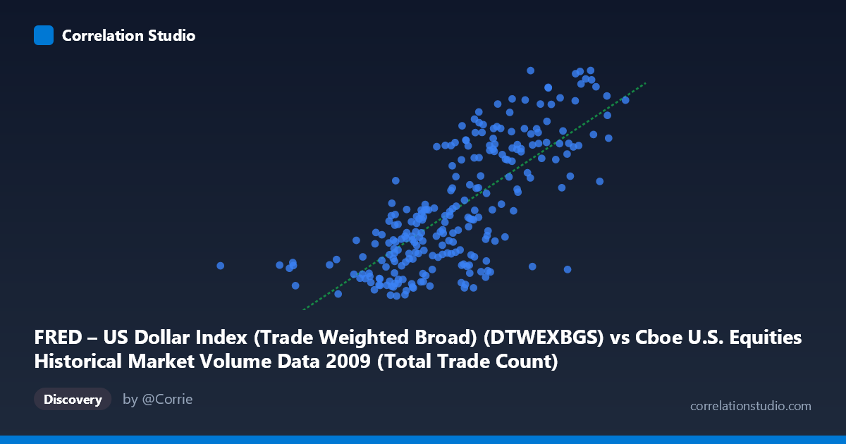
FRED – US Dollar Index (Trade Weighted Broad) (DTWEXBGS) vs Cboe U.S. Equities Historical Market Volume Data 2009 (Total Trade Count)
- Pearson correlation (r)
- 0.7435
- Spearman correlation
- 0.7331
- p-value
- 0
- Sample size (n)
- 248
- 95% confidence interval
- 0.6821 to 0.7945
- Granger causality
- None
- Granger optimal lag
- 1
AI analysis
Scatterplot Analysis: US Dollar Index vs. Total Trade Count (2009)
Relationship Overview
The scatterplot reveals a positive, moderately strong linear relationship between the US Dollar Index (Trade Weighted Broad) on the X-axis and Total Trade Count on the Y-axis across 248 trading days in 2009. As the dollar index increases, trade counts tend to rise as well, with the linear regression equation y = 5.165×10⁻⁶x + 82.923 capturing this upward trend. The relationship appears reasonably consistent across the middle range of the data, though there is notable scatter, particularly at the lower end of the X-axis where trade counts cluster between roughly 91–94 despite a wide spread in dollar index values. The overall visual pattern is consistent with a moderate positive association rather than a tight deterministic link.
Correlation Strength and Statistical Interpretation
The Pearson correlation of r = 0.7435 indicates a moderately strong positive association, and the R² of 0.5528 means that approximately 55.3% of the variance in Total Trade Count is explained by variation in the Dollar Index — a meaningful but far from complete explanation, leaving nearly 45% of variance attributable to other factors. The 95% confidence interval of [0.6821, 0.7945] is relatively tight, reflecting the reasonably large sample of n = 248, and the p-value of essentially zero confirms the relationship is highly statistically significant and extremely unlikely to be a chance artifact. However, statistical significance alone does not imply practical or causal meaningfulness. The Granger causality results are notably absent in both directions — X→Y (F = 0.9469, p = 0.3315) and Y→X (F = 0.3026, p = 0.5828) — meaning that despite the strong contemporaneous correlation, neither variable temporally predicts the other at a 1-period lag. This is a critical caveat: the two variables move together, but neither leads the other in a predictive sense.
Notable Patterns, Clusters, and Outliers
Several structural features stand out in the data. There is a dense cluster of points at lower X values (roughly 1,900,000–2,400,000) that predominantly occupy the lower Y range (91–96), suggesting a regime of lower dollar index values coinciding with lower trade activity — likely reflecting the early 2009 period of market stress and recovery. Conversely, high-X observations (3,500,000–4,134,000) consistently map to high Y values (100–106), forming a distinct upper-right cluster that anchors the positive slope. The point at approximately (629,671, 92.87) appears as a notable low-end outlier on the X-axis, far removed from the bulk of the distribution (mean X ≈ 2,673,918), which could reflect an anomalous trading day or data recording issue and may have modest leverage on the regression. There is also a suggestion of heteroscedasticity — variance in Y appears somewhat larger in the middle X range than at the extremes — which could mildly violate linear regression assumptions.
Confounding Factors and Interpretive Caveats
The 2009 timeframe is crucial context: this period encompassed the tail end of the Global Financial Crisis and subsequent market recovery, meaning both variables were simultaneously influenced by macro regime shifts — credit conditions, Federal Reserve policy, risk sentiment, and institutional positioning. This shared dependence on a third driver (macro environment/risk appetite) is a classic confounding scenario, likely inflating the observed correlation without implying any direct mechanical link between dollar strength and trade counts. Additionally, the Granger non-causality result reinforces that the correlation is likely spurious or driven by a common underlying factor rather than a direct channel. The broad dollar index reflects international currency dynamics, while trade count reflects domestic equity market microstructure activity — these operate through fundamentally different mechanisms. The large population N of 3,232 versus sample n of 248 also warrants attention; if the sample is not fully representative of the population distribution, estimates may be biased.
Actionable Insights and Further Investigation
Given the strong contemporaneous correlation but absence of Granger causality, the most productive next step would be to identify the latent common driver — likely a risk sentiment index (e.g., VIX), equity market returns (S&P 500), or Federal Reserve balance sheet activity — and run a partial correlation or multivariate regression controlling for these factors to assess whether the dollar-trade count relationship survives. It would also be valuable to extend the analysis beyond 2009 to test whether this correlation is a structural feature of markets or an artifact of the crisis-recovery regime. Testing for non-linear specifications (e.g., polynomial or piecewise regression) and formally diagnosing heteroscedasticity would improve model reliability. Finally, disaggregating trade counts by exchange or asset class (Cboe-specific vs. TRF) may reveal whether the relationship is concentrated in particular market segments, providing more targeted and actionable intelligence for market microstructure research or trading strategy development.
X dataset: Cboe U.S. Equities Historical Market Volume Data 2009
Y dataset: FRED – US Dollar Index (Trade Weighted Broad)
Part of experiment: Daily - Cboe U.S. Equities Historical Market Volume Data 2009 vs FRED – US Dollar Index (Trade Weighted Broad)