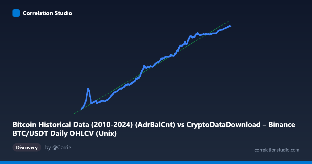
Bitcoin Historical Data (2010-2024) (AdrBalCnt) vs CryptoDataDownload – Binance BTC/USDT Daily OHLCV (Unix)
- Pearson correlation (r)
- 0.9877
- Spearman correlation
- 0.992
- p-value
- 0
- Sample size (n)
- 3191
- 95% confidence interval
- 0.9868 to 0.9885
- Granger causality
- None
- Granger optimal lag
- 10
- Time coverage
- 2017-08-17 to 2026-05-20
AI analysis
Analysis: Bitcoin Address/Time Metric vs. BTC/USDT Metric
1. Overview of the Relationship
The scatterplot depicts a strikingly tight, monotonically increasing relationship between the X variable (timestamp-indexed, spanning August 2017 to mid-2026) and Y (ranging ~18.8M to ~57M). Given that X is effectively a time index (Unix timestamps in milliseconds) and Y is a large, steadily growing count, this plot is best understood as a long-run growth trend over time rather than a relationship between two independent economic signals. The data points trace a smooth, upward-sloping curve with very little scatter around the fitted line, indicating that Y has grown almost deterministically as time has progressed.
2. Strength, Direction, and Statistical Confidence
The correlation is very strong and positive (r = 0.9877, r² = 0.9755), meaning 97.6% of the variance in Y is explained by X in a simple linear model. The 95% confidence interval [0.9868, 0.9885] is extremely narrow, and the p-value is effectively 0 — both consistent with a large sample (n = 3,191) and a highly stable, non-noisy trend rather than a fragile statistical artifact. Practically, this tells us the two series co-move almost in lockstep over the sampled period.
However, the Granger causality results are important context: neither variable Granger-causes the other (X→Y: p = 0.559; Y→X: p = 0.454). This indicates that despite the strong contemporaneous correlation, neither series has predictive power over the other's future values beyond what's already captured in its own past. This is a classic signature of two variables that are both driven by a common underlying trend (time/adoption growth) rather than one causally leading the other in a lagged, dynamic sense.
3. Patterns, Clusters, and Non-linearity
Several features stand out: - Regime-like clustering: Sample points show distinct "bands" — e.g., 2017-2019 values cluster around 19-28M, 2020-2021 around 30-38M, 2023-2024 around 48-53M, and 2025-2026 around 54-57M. This suggests the growth is not perfectly linear but has periods of faster and slower increase (consistent with Bitcoin adoption S-curves or halving-cycle effects). - Flattening at the upper range: Y appears to be approaching an asymptote near 55-57M in the most recent data (2025-2026), suggesting decelerating growth — a potential saturation or logistic pattern rather than pure linear growth. - Compression in early years: The 2017-2019 points show relatively small Y changes despite meaningful time elapsed, hinting at slower early-stage adoption. - These patterns imply the true relationship may be better fit by a logistic, power, or piecewise curve rather than a straight line, even though the linear R² is already very high.
4. Confounding Factors and Caveats
- Spurious trend correlation: Because X is essentially a time proxy, this is a classic case where two unrelated (or indirectly related) growing time series will show high correlation simply due to shared temporal trend — not necessarily a meaningful causal or economic linkage between "address count" and "OHLCV-derived" metrics. - Autocorrelation: Both series are highly autocorrelated (each day resembles the prior day), which inflates r and r² and violates independence assumptions underlying the p-value calculation — the true "effective sample size" is much smaller than 3,191. - Non-stationarity: Neither series is likely stationary (both trend upward over time), which is precisely why standard Granger causality tests fail to find lead-lag structure — the test assumes stationarity, and its non-significance may reflect model misspecification rather than genuine lack of relationship. - Metric ambiguity: The axis labels are unusually cross-referenced (X labeled as "AdrBalCnt" from a CDD OHLCV dataset; Y labeled as OHLCV data from a different Bitcoin metrics dataset), suggesting possible mislabeling or metadata mismatch that should be verified before drawing substantive conclusions.
5. Recommendations for Further Investigation
- Detrend or difference both series (e.g., use daily/weekly returns or log-differences) and re-run correlation and Granger tests to check whether the relationship holds after removing the shared time trend — this is the standard remedy for spurious trend correlation. - Test for cointegration (e.g., Engle-Granger or Johansen test) given both series appear non-stationary and trending; this would clarify whether a genuine long-run equilibrium relationship exists. - Fit a logistic/S-curve model instead of linear regression, given visual evidence of deceleration at the upper end, to better capture the true functional form and improve extrapolation accuracy. - Verify data labeling/provenance to confirm what X and Y actually represent, since the current axis descriptions appear to reference overlapping/inconsistent dataset sources. - Segment by cycle (e.g., pre/post-halving periods) to test whether the growth rate itself correlates with known Bitcoin market cycles, which may offer more actionable, structurally grounded insights than the raw pooled correlation.
X dataset: CryptoDataDownload – Binance BTC/USDT Daily OHLCV
Y dataset: Bitcoin Historical Data (2010-2024)
Part of experiment: Bitcoin - CryptoDataDownload – Binance BTC/USDT Daily OHLCV vs Bitcoin Historical Data (2010-2024)