FRED – 5-Year Breakeven Inflation Rate (T5YIE) vs 10-Year US Treasury Constant Maturity Rate (FRED) (DGS10)
- Pearson correlation (r)
- 0.4248
- Spearman correlation
- 0.5223
- p-value
- 0
- Sample size (n)
- 5852
- 95% confidence interval
- 0.4036 to 0.4456
- Granger causality
- None
- Granger optimal lag
- 1
AI analysis
Analysis: 5-Year Breakeven Inflation Rate vs. 10-Year Treasury Yield
Relationship Overview
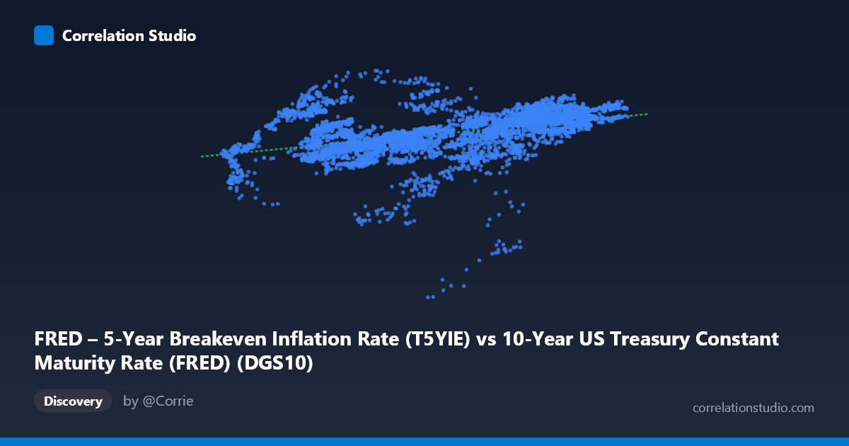
The scatterplot reveals a modest positive relationship between the 5-Year Breakeven Inflation Rate (X) and the 10-Year Treasury Constant Maturity Rate (Y), described by the regression line y = 0.209x + 1.312. As inflation expectations rise, 10-year Treasury yields tend to rise as well — an economically intuitive finding, since bond markets typically demand higher nominal yields when inflation expectations increase. However, the relationship is clearly noisy, with substantial vertical scatter at nearly every value of X. The data spans over two decades (2003–2026), capturing multiple economic regimes including the post-GFC low-rate era, the COVID shock, and the 2022–2023 inflation surge, which likely accounts for the wide dispersion visible in the plot.
Correlation Strength and Statistical Significance
The Pearson correlation of r = 0.4248 indicates a moderate positive association, but the r² of 0.1805 means only ~18% of the variance in 10-year yields is explained by breakeven inflation rates — leaving roughly 82% of yield variation attributable to other forces. The 95% confidence interval of [0.4036, 0.4456] is narrow given the large paired sample (n = 5,852), and the p-value is effectively zero, confirming this correlation is highly unlikely to be a statistical artifact. That said, statistical significance here is largely a function of the enormous sample size rather than a strong effect size. The Granger causality tests are notably inconclusive in both directions (X→Y: F = 2.51, p = 0.11; Y→X: F = 0.32, p = 0.57), meaning neither variable reliably predicts the other one period ahead after accounting for their own history. This absence of temporal predictive direction is an important caveat: the correlation is contemporaneous rather than predictive.
Patterns, Clusters, and Notable Features
The sample points reveal several structural features. There is a dense cluster roughly between X = 1.5–3.0 and Y = 1.5–2.2, consistent with the low-inflation, low-yield environment that dominated 2003–2019. A second, more dispersed cluster appears at X = 4.0–5.0 with Y = 2.0–2.6, likely representing the post-2021 inflationary episode when both breakeven rates and nominal yields surged. The Y-axis range extends down to -2.24, suggesting periods of negative inflation expectations (deflationary fears, plausibly during the 2008–2009 GFC or early COVID), while some extreme Y values near 3.5+ reflect the 2022–2023 rate-hiking cycle. The relationship appears non-linear or regime-dependent — the slope appears steeper at low breakeven values and flatter at higher ones, suggesting diminishing sensitivity at elevated inflation expectations.
Confounding Factors and Caveats
Several confounders limit causal interpretation. Federal Reserve policy is a dominant independent driver of both variables simultaneously — rate hikes compress real yields and affect inflation expectations in tandem, creating spurious co-movement. Risk premia and term premia embedded in the 10-year yield fluctuate with global demand for safe assets (e.g., flight-to-quality episodes during crises), decoupling yields from inflation expectations. The two-decade time span introduces structural breaks — the zero-lower-bound era (2009–2015), quantitative easing programs, and the post-COVID inflation shock are fundamentally different economic regimes that may each have distinct internal dynamics, making pooled regression misleading. Additionally, breakeven rates themselves reflect liquidity premia in TIPS markets, not pure inflation expectations, adding measurement noise to X.
Actionable Insights and Further Investigation
Given the regime-dependent appearance of the data, a regime-switching model or rolling-window correlation analysis would help determine whether the X-Y relationship strengthened or weakened across economic cycles. Researchers should consider controlling for the Federal Funds Rate, real GDP growth, and credit spreads to isolate the partial relationship between inflation expectations and long-term yields. Testing non-linear specifications (e.g., piecewise regression, spline models) could better capture the apparent heteroscedasticity across the X range. Finally, extending the Granger analysis to multiple lags (beyond the optimal lag-1 tested) and incorporating a VAR framework with additional macroeconomic variables would provide a more robust assessment of whether inflation expectations genuinely lead or lag changes in Treasury yields across different time horizons.
X dataset: 10-Year US Treasury Constant Maturity Rate (FRED)
Y dataset: FRED – 5-Year Breakeven Inflation Rate
Part of experiment: Daily - 10-Year US Treasury Constant Maturity Rate (FRED) vs FRED – 5-Year Breakeven Inflation Rate