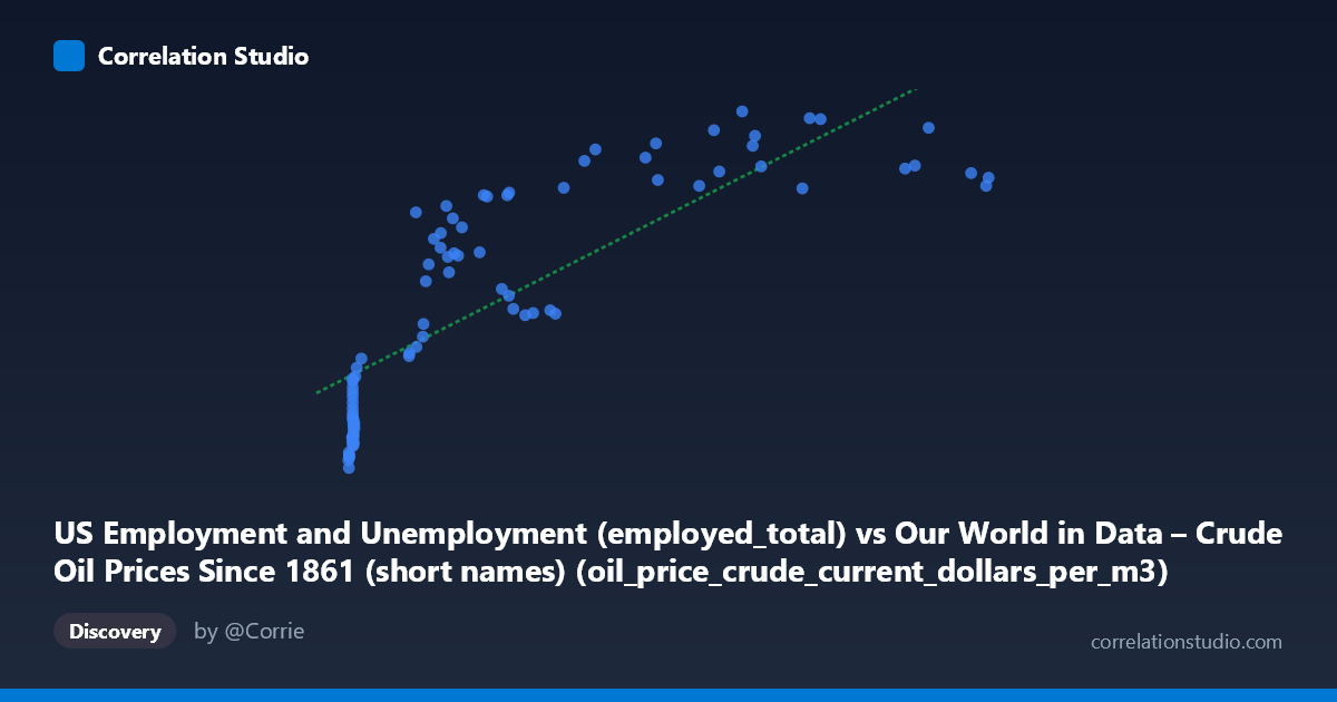
US Employment and Unemployment (employed_total) vs Our World in Data – Crude Oil Prices Since 1861 (short names) (oil_price_crude_current_dollars_per_m3)
- Pearson correlation (r)
- 0.8145
- Spearman correlation
- 0.9155
- p-value
- 0
- Sample size (n)
- 85
- 95% confidence interval
- 0.7277 to 0.8756
- Granger causality
- None
- Granger optimal lag
- 10
- Time coverage
- 1941-01-01 to 2025-01-01
- Recomputed on refreshed data
- 2026-10-09 (r was 0.81)
AI analysis
Analysis: Crude Oil Prices vs. US Total Employment (1941–2024)
1. What the Visualization Reveals
The scatterplot displays a positive relationship between crude oil prices (in current dollars per cubic meter) on the X-axis and total US employment on the Y-axis, spanning over eight decades of annual data. The overall trend is upward — as oil prices have risen historically, so too has total US employment — though the relationship is clearly not uniform across the range. At low oil price values (roughly below $100/m³), employment figures cluster tightly in a lower band, while higher oil prices correspond to a wide spread of employment outcomes. This fan-shaped dispersion suggests that the linear model captures a general trend but misses meaningful structural variation in the data.
2. Correlation Strength, Direction, and Causality
The Pearson correlation of r = 0.81 indicates a strong positive association, and the R² of 0.6561 means that approximately 65.6% of the variance in US employment is statistically explained by crude oil prices in this bivariate linear model — a substantial share for a single predictor. The 95% confidence interval for r of [0.72, 0.87] is reasonably tight, reinforcing that the correlation is not a statistical artifact, and the p-value of effectively zero confirms the relationship is highly significant at conventional thresholds. However, the Granger causality tests tell a more cautionary story: neither direction of temporal prediction is statistically significant (X→Y: F = 1.10, p = 0.38; Y→X: F = 1.40, p = 0.21), even at an optimal lag of 10 periods. This means that knowing past oil prices does not meaningfully improve forecasts of future employment beyond what employment's own history already provides, and vice versa. The correlation is real, but it does not reflect a predictive or causal temporal mechanism in either direction.
3. Notable Patterns, Clusters, and Non-Linearity
Three structural features stand out visually. First, there is a dense cluster of points at very low X values (roughly $6–$20/m³) corresponding to pre-1970s oil pricing, where employment ranges from approximately 50,000 to 85,000 (presumably thousands), forming a tight grouping that anchors the lower-left of the plot. Second, the middle range of oil prices ($80–$350/m³) shows considerable vertical scatter, with employment values spanning nearly the full Y-axis range — indicating that similar oil price levels coincided with very different employment environments across different historical eras. Third, at the high end of oil prices (above $500/m³), employment values paradoxically begin to plateau or even decline slightly, hinting at a logarithmic or concave relationship rather than a linear one. Critically, the note that Spearman ρ exceeds Pearson r formally flags this non-linearity: a logarithmic or polynomial regression would almost certainly provide a better statistical fit than the current linear model (y = 146.58x + 78,334.8).
4. Confounding Factors and Interpretive Caveats
This correlation is almost certainly driven by a shared common cause: long-run time trends. Both crude oil prices and US total employment have generally increased over the 1941–2024 period, the former due to energy market evolution, geopolitical shocks (OPEC embargoes, Gulf Wars, COVID-19 supply disruptions), and inflation, and the latter due to US population growth, labor force expansion, and economic development. This makes the correlation largely spurious in a causal sense — two variables both trending upward over time will naturally correlate strongly without one causing the other. Additionally, oil price is denominated in nominal (current) dollars, so inflationary growth inflates prices independently of real energy market dynamics. Employment figures also do not adjust for labor force participation rates or population size, meaning long-run demographic expansion mechanically drives Y upward. The Granger test's null results reinforce this interpretation: the statistical link evaporates once temporal structure is properly accounted for.
5. Actionable Insights and Further Investigation
Given these findings, several analytical steps are warranted. First, detrend both series (e.g., first-differencing or HP filtering) before re-examining correlation to strip out the shared time trend and test whether a meaningful relationship persists in the fluctuations around trend. Second, replace nominal oil prices with inflation-adjusted (real) oil prices to separate genuine energy price signals from monetary inflation. Third, fit a logarithmic regression (ln(X) → Y) given the Spearman-Pearson discrepancy, which would likely better capture the diminishing marginal relationship visible at high oil price values. Fourth, extend the Granger causality analysis using shorter, theoretically motivated lags (1–3 years) rather than the data-selected 10-period lag, and consider VAR models incorporating GDP, inflation, and population as controls. Finally, it would be worth examining sub-period analyses (e.g., pre- vs. post-1973 oil shock, or pre- vs. post-2000) to test whether the relationship is stable across different energy and labor market regimes — the current aggregate correlation likely masks substantial structural heterogeneity across time.
X dataset: Our World in Data – Crude Oil Prices Since 1861 (short names)
Y dataset: US Employment and Unemployment
Part of experiment: Yearly - Our World in Data – Crude Oil Prices Since 1861 (short names) vs US Employment and Unemployment