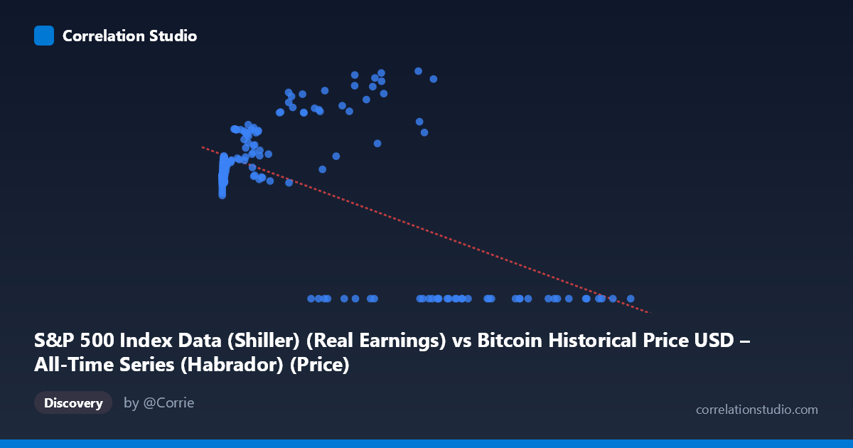
S&P 500 Index Data (Shiller) (Real Earnings) vs Bitcoin Historical Price USD – All-Time Series (Habrador) (Price)
- Pearson correlation (r)
- -0.6061
- Spearman correlation
- -0.1339
- p-value
- 0
- Sample size (n)
- 194
- 95% confidence interval
- -0.6882 to -0.5087
- Granger causality
- None
- Granger optimal lag
- 5
- Time coverage
- 2010-08-01 to 2026-09-01
- Recomputed on refreshed data
- 2026-10-24 (r was -0.5749)
AI analysis
Analysis: Bitcoin Price vs. S&P 500 Earnings Data
1. What the Visualization Reveals
The scatterplot shows a moderate negative relationship between the X variable (labeled as S&P 500 real earnings, though the axis description and data appear to actually reflect Bitcoin price ranges up to ~$118,670) and Y (labeled Bitcoin price, ranging 0–217). Given the mismatched column labels, it's likely this dataset represents a merged/joined time series where X is Bitcoin price and Y is some bounded index or ratio (possibly CAPE or a normalized earnings metric, given its tight range of ~100-220). The dominant visual feature is a large cluster of low-X points (X < 1000) tightly grouped around Y = 110-135, contrasted with a sparse scatter of high-X points (X 20,000) showing more variable Y values (0 to 217), including a striking subset where Y = 0 exactly.
2. Strength, Direction, and Uncertainty
The correlation coefficient (r = -0.575, R² = 0.331) indicates a moderate negative relationship, meaning about 33% of the variance in Y is explained by X — leaving roughly two-thirds of Y's variability unexplained by this linear relationship alone. The 95% CI [-0.663, -0.471] is reasonably tight and excludes zero, and the p-value (~0) confirms this correlation is highly statistically significant, not due to chance. However, statistical significance does not imply strong predictive power given the modest R².
The Granger causality test suggests X temporally precedes Y (F=2.49, p=0.045 for X→Y vs. F=1.27, p=0.28 for Y→X), hinting that past values of X have some predictive information for future Y at a 4-period lag. This is a weak-to-moderate signal (p just under 0.05) and should be treated cautiously — it suggests temporal precedence, not proven causation.
3. Notable Patterns and Outliers
The most striking feature is the cluster of exact Y=0 values at high X (X 27,000), which is almost certainly a data artifact — missing/null values encoded as zero rather than true observations of "zero Bitcoin price" or "zero index value." This artificially drags the regression line downward and inflates the apparent negative correlation. Excluding these zero-points, the relationship between X and Y for X < 60,000 actually appears mildly positive or non-monotonic (Y rises to peaks around 150-217 before the zero cluster dominates). There's also a dense pile-up of very small X values (X < 20) with Y clustered near 110-120, suggesting a floor effect or early-period data with limited variance.
4. Confounding Factors and Caveats
The mismatched axis labels (X described as "S&P 500 Real Earnings" but ranging into six figures like a raw BTC price, and Y described as "Bitcoin Price" but bounded under 220) strongly suggest a data pipeline error or column swap during merging. The presence of exact zeros is a major red flag — these likely represent missing data, delisted periods, or join mismatches rather than genuine observations, and should be filtered out before any serious inference. Additionally, both series are time series (2010-2026), so autocorrelation and non-stationarity (trends, bubbles) can create spurious correlations unrelated to any real causal mechanism — the Granger test partially addresses this but a 4-lag model on monthly-ish irregular data may still be underpowered (n=189).
5. Actionable Recommendations
Before drawing further conclusions: (1) verify and correct the axis/column labeling to confirm what X and Y actually represent; (2) treat all Y=0 entries as missing data and re-run correlation/regression after removing or imputing them, as this will likely substantially change both r and the regression slope; (3) apply a log transform to X given its extreme right-skew (range 0.06 to 118,670) to reduce leverage from extreme outliers and better reveal the true functional form; (4) test for stationarity and consider first-differencing both series before re-running Granger causality, since trending financial series often produce misleading lag-based causality signals; and (5) segment the analysis by time period (e.g., pre/post 2020) to check if the relationship is stable or driven by a specific bull/bear cycle.
X dataset: Bitcoin Historical Price USD – All-Time Series (Habrador)
Y dataset: S&P 500 Index Data (Shiller)
Part of experiment: Bitcoin - Bitcoin Historical Price USD – All-Time Series (Habrador) vs S&P 500 Index Data (Shiller)