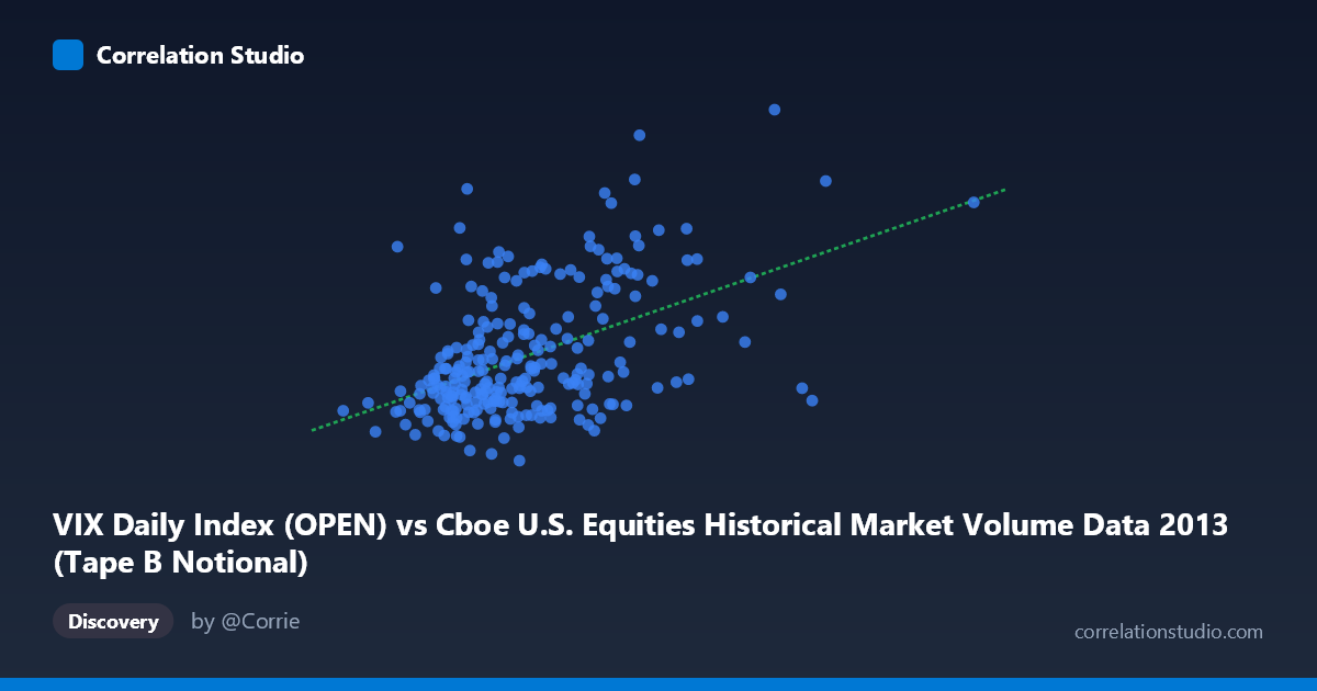
VIX Daily Index (OPEN) vs Cboe U.S. Equities Historical Market Volume Data 2013 (Tape B Notional)
- Pearson correlation (r)
- 0.4869
- Spearman correlation
- 0.4394
- p-value
- 0
- Sample size (n)
- 252
- 95% confidence interval
- 0.3866 to 0.5758
- Granger causality
- None
- Granger optimal lag
- 1
AI analysis
Scatterplot Analysis: VIX Open vs. Tape B Notional Volume (2013)
Relationship Overview
The scatterplot reveals a positive relationship between the CBOE VIX Daily Index (Open) values on the X-axis and Tape B Notional trading volume on the Y-axis across 252 trading days in 2013. The linear regression equation (y = 7.78×10⁻¹⁰x + 11.28) confirms this upward trend, suggesting that as market volume (measured in notional terms) increases, VIX open values tend to rise correspondingly. This is conceptually intuitive: higher trading volumes in U.S. equity markets are often associated with periods of elevated uncertainty or volatility, which the VIX is specifically designed to capture. However, the relationship is far from deterministic, and the scatter around the regression line is substantial, indicating considerable noise in the association.
Correlation Strength and Statistical Framing
The Pearson correlation of r = 0.487 indicates a moderate positive association, but the explained variance tells a more sobering story: r² = 0.237 means that only 23.7% of the variance in VIX open values is accounted for by Tape B notional volume, leaving roughly 76% attributable to other factors. The 95% confidence interval for r [0.387, 0.576] is reasonably narrow given the sample size of 252, and the p-value of 2.22×10⁻¹⁶ confirms the correlation is highly statistically significant, effectively ruling out chance as an explanation. That said, statistical significance here is partly a function of the large underlying population (N = 3,780), and significance should not be conflated with practical magnitude. Critically, the Granger causality tests find no significant directional predictive relationship in either direction — neither does volume predict future VIX (F = 1.61, p = 0.21), nor does VIX predict future volume (F = 0.40, p = 0.53). This means the correlation is contemporaneous rather than temporally predictive, undermining any strategy that would use one variable to forecast the other.
Patterns, Clusters, and Outliers
The sample points reveal several noteworthy structural features. The bulk of observations cluster in a core region — roughly X values between 2.9×10⁹ and 4.5×10⁹ and Y values between 12 and 16 — suggesting a relatively stable baseline regime for most of 2013. However, there are clear high-leverage outliers worth flagging: the point near (5.19×10⁹, 19.01) and another near (5.19×10⁹, 15.90) indicate episodes of unusually high volume coinciding with elevated VIX readings, likely corresponding to specific market stress events during 2013 (such as the May "Taper Tantrum" period). Conversely, a point at approximately (7.30×10⁹, 13.12) represents an extreme volume observation with a surprisingly low VIX value, which defies the general trend and may represent an end-of-year volume surge under calm market conditions. The X range extends to nearly 9.2×10⁹, suggesting right-skewed volume data, and the nonlinear dispersion of residuals hints that a log-linear or segmented model might better capture the relationship than a simple linear fit.
Confounding Factors and Interpretive Caveats
Several important caveats apply. First, the axes appear to be swapped from conventional expectations: VIX is plotted on the X-axis while Tape B notional volume appears on Y, which is an unconventional framing since VIX is more naturally treated as a dependent market sentiment indicator. This labeling inversion warrants careful verification before drawing directional conclusions. Second, Tape B notional volume represents only a subset of total U.S. equity market volume (specifically NYSE American and regional exchange-listed securities), which may not fully represent aggregate market activity. Third, 2013 was a distinctly low-volatility, bull-market year (VIX averaged well below historical norms), meaning this correlation may not generalize to other market regimes — particularly high-stress periods where the VIX-volume relationship could become much stronger or structurally different. Finally, common drivers such as macroeconomic announcements, Federal Reserve communications, or earnings seasons could simultaneously elevate both VIX and volume, creating spurious correlation without a true causal mechanism between the two variables themselves.
Actionable Insights and Further Investigation
Given the moderate but statistically robust correlation and the absence of Granger causality, practitioners should treat this relationship as a coincident indicator rather than a predictive signal. Several next steps would strengthen the analysis: (1) Extend the time series across multiple years to test whether 2013's low-volatility regime suppresses what might be a stronger relationship during stress periods — a rolling-window correlation analysis would reveal regime dependence; (2) Disaggregate by market event type (FOMC days, earnings announcements, macro data releases) to identify whether specific catalysts drive both variables simultaneously, which would help isolate confounding; (3) Test non-linear models (log transformation of volume, quantile regression, or piecewise regression) given the apparent heteroscedasticity and the outlier structure; (4) Compare Tape A, B, and C notional volumes against VIX to determine whether the relationship is specific to Tape B or reflects a market-wide phenomenon; and (5) Incorporate lagged VIX levels and implied volatility term structure to better isolate whether volume changes (rather than levels) carry more predictive information about near-term volatility expectations.
X dataset: Cboe U.S. Equities Historical Market Volume Data 2013
Y dataset: VIX Daily Index
Part of experiment: Daily - Cboe U.S. Equities Historical Market Volume Data 2013 vs VIX Daily Index