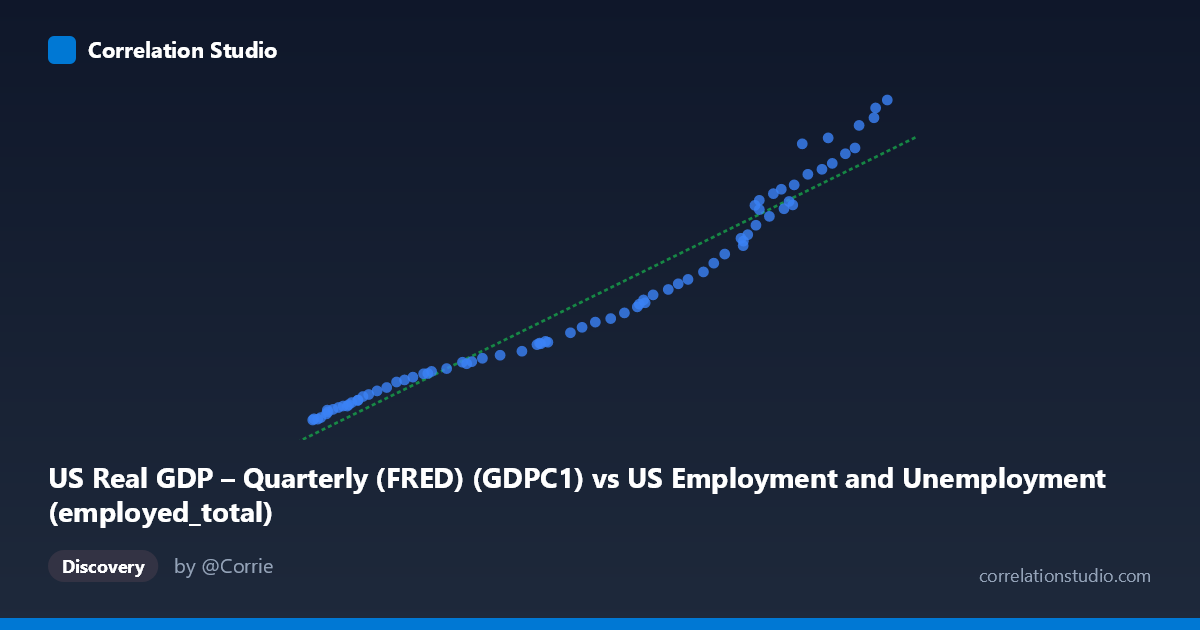
US Real GDP – Quarterly (FRED) (GDPC1) vs US Employment and Unemployment (employed_total)
- Pearson correlation (r)
- 0.9735
- Spearman correlation
- 0.9979
- p-value
- 0
- Sample size (n)
- 79
- 95% confidence interval
- 0.9588 to 0.983
- Granger causality
- None
- Granger optimal lag
- 10
AI analysis
Analysis: US Real GDP vs. Total Employment
Relationship Overview
The scatterplot reveals a strong, positive, and approximately linear relationship between US Real GDP (quarterly, in billions of chained 2017 dollars) and total US employment. As GDP rises from roughly $57,000B to $163,000B, total employment climbs from approximately 2,200 to 23,500 (thousands or millions, depending on units). The data points cluster tightly around the regression line y = 0.179x − 9,079, indicating that these two macroeconomic series move together in a highly consistent, near-monotonic fashion across the 1947–2025 observation window. This is an intuitive finding: a growing economy tends to generate more jobs, and a larger workforce tends to produce more output.
Correlation Strength and Statistical Significance
The correlation is exceptionally strong at r = 0.9737, with r² = 0.9481, meaning that approximately 94.8% of the variance in total employment is statistically explained by variation in Real GDP within this sample. The 95% confidence interval for r is tight at [0.9591, 0.9831], confirming high precision in the estimate, and the p-value of effectively zero (p ≈ 0, n = 79) rules out chance as an explanation. However, despite this impressive correlation, the Granger causality tests reveal no statistically significant predictive direction in either direction — neither GDP predicting employment (F = 1.69, p = 0.111) nor employment predicting GDP (F = 1.63, p = 0.128) survives the threshold at the optimal 10-period lag. This is a critical nuance: the two series are tightly co-integrated over time but neither reliably leads the other at this lag structure, suggesting they evolve largely contemporaneously as joint outcomes of broader economic forces.
Patterns, Clusters, and Notable Features
The scatterplot exhibits a relatively clean linear sweep with no dramatic outliers, but closer inspection suggests a few structural features worth noting. The lower-left cluster (GDP ~57,000–75,000; employment ~2,200–5,000) likely represents the early postwar decades when both the economy and labor force were smaller in absolute terms. The upper-right region (GDP $140,000B; employment $15,000) reflects the modern era of a large, mature economy. There may be slight heteroscedasticity — variance in employment appears to fan out modestly at higher GDP values — which could indicate that the relationship is not perfectly linear across all eras, possibly reflecting structural labor market shifts (automation, labor force participation trends, sectoral transitions). A few points at the extreme upper end (GDP ~$160,000B+) appear to sit very close to or slightly above the regression line, suggesting employment grew robustly relative to GDP in recent years.
Confounding Factors and Caveats
Several important caveats temper a causal interpretation. First, both series are strongly trended over time, meaning much of the observed correlation may reflect shared secular growth trends rather than a direct structural relationship — a classic spurious correlation risk with non-stationary time series. The absence of Granger causality reinforces this concern. Second, data aggregation matters: GDP is measured quarterly while employment is annual, and the merging of these series introduces temporal mismatch. Third, composition changes over 78 years are substantial — the nature of employment (part-time vs. full-time, gig economy, productivity per worker) and the composition of GDP (services vs. manufacturing) have shifted dramatically, meaning the same regression slope may not hold uniformly across subperiods. Fourth, population growth is a common driver of both variables, acting as a significant omitted confounder.
Actionable Insights and Further Investigation
Given the strength of the association but the absence of Granger causality, the most productive next steps would include: (1) testing the relationship on first-differenced or detrended data (e.g., GDP growth rates vs. employment growth rates) to isolate cyclical dynamics from secular trends and reduce spurious correlation risk; (2) conducting subperiod analysis (pre/post-1990, pre/post-2008 financial crisis) to test whether the slope has shifted, which would have implications for interpreting productivity growth; (3) introducing control variables such as working-age population, labor force participation rate, and average hours worked to better isolate the independent GDP–employment link; and (4) exploring non-linear or threshold models to test whether the relationship changes character at different phases of the business cycle. The high r² makes this a useful forecasting baseline, but policymakers and researchers should treat it as descriptive co-movement rather than evidence of a clean causal mechanism.
X dataset: US Employment and Unemployment
Y dataset: US Real GDP – Quarterly (FRED)
Part of experiment: Yearly - US Employment and Unemployment vs US Real GDP – Quarterly (FRED)