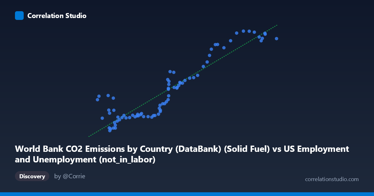
World Bank CO2 Emissions by Country (DataBank) (Solid Fuel) vs US Employment and Unemployment (not_in_labor)
- Pearson correlation (r)
- 0.9245
- Spearman correlation
- 0.8781
- p-value
- 0
- Sample size (n)
- 80
- 95% confidence interval
- 0.8844 to 0.951
- Granger causality
- None
- Granger optimal lag
- 10
AI analysis
Scatterplot Analysis: Solid Fuel CO2 Emissions vs. US Labor Force Non-Participation
1. Overall Relationship The scatterplot reveals a strong positive relationship between World Bank solid fuel CO2 emissions and the number of Americans not in the labor force. As solid fuel CO2 emissions increase (X-axis, ranging from ~38,590 to ~99,587 units), the count of non-labor-force participants (Y-axis, ranging from ~9,555 to ~31,154 thousand) rises substantially. The linear regression equation y = 0.377x − 5,174.84 captures this upward trend, suggesting that for every unit increase in solid fuel emissions, approximately 0.377 additional units of non-labor-force participation are associated. Given the time coverage spans 1941–2020, both variables are almost certainly being driven by shared long-run secular trends — namely, post-war economic and demographic expansion — rather than any direct causal mechanism between them.
2. Correlation Strength and Statistical Framing The Pearson correlation of r = 0.9245 is very strong, and the R² of 0.8546 indicates that approximately 85.5% of the variance in non-labor-force participation is statistically explained by solid fuel CO2 emissions within this linear model. The 95% confidence interval for r of [0.8844, 0.9510] is notably tight, reflecting high precision in the estimate across the n = 80 paired observations, and the p-value of effectively 0 confirms the result is highly statistically significant. However, the Granger causality tests tell a critically important story: neither direction of temporal predictive causality is significant (X→Y: F = 0.63, p = 0.78; Y→X: F = 1.02, p = 0.44), even at an optimal lag of 10 periods. This means that despite the impressive correlation, neither variable meaningfully predicts future changes in the other once past values are accounted for. The high r² reflects shared time-trend confounding, not genuine predictive or causal linkage.
3. Notable Patterns, Clusters, and Outliers The data exhibit a broadly monotonic positive trend but with visually distinct clustering behavior. A lower-left cluster of points (X: 38,000–55,000; Y: 9,500–14,000) corresponds to earlier decades (likely 1940s–1960s), where both emissions and non-participation were relatively low, and the points are tightly packed with modest spread. A middle transitional zone (X: 55,000–75,000; Y: 12,000–25,000) shows increasing scatter and variance — the funnel-like spread widens here, hinting at heteroscedasticity. The upper-right cluster (X: 80,000–99,587; Y: 27,000–31,154) corresponds to recent decades, where non-labor-force participation plateaus somewhat even as emissions remain high, producing slight compression at the upper range. A few notable outliers appear in the lower-middle X range with surprisingly high Y values — points such as (38,590; 16,274), (39,100; 17,031), (42,230; 17,184), and (43,990; 16,616) show relatively low emissions but elevated non-participation, possibly reflecting early post-war demographic anomalies or measurement artifacts worth investigating.
4. Confounding Factors and Caveats This correlation is a near-textbook example of spurious correlation driven by mutual time trends. Both solid fuel CO2 emissions and non-labor-force participation grew substantially over the 80-year period covered (1941–2020) due to entirely independent forces: emissions reflect industrialization, energy infrastructure growth, and later partial decarbonization; non-labor-force participation reflects population growth, aging demographics, rising rates of retirement, student enrollment, and disability. Population size is the most likely common driver — a larger population both burns more fuel and contributes more non-participants by sheer scale. Additionally, the dataset pairing itself is conceptually unusual: one variable is drawn from a global CO2 emissions dataset (World Bank) while the other is a US-specific labor metric (BLS), meaning geographic scope mismatch further undermines any causal interpretation. The widening variance in the middle range also suggests the linear model may not be the optimal functional form across all periods.
5. Actionable Insights and Further Investigation Given the absence of Granger causality and the strong likelihood of spurious correlation, the most important next step is detrending both series — removing the shared long-run trend (e.g., via first-differencing or HP filtering) and re-examining whether any residual correlation remains. Researchers should also control for population size by normalizing both variables on a per-capita basis, which would likely substantially reduce or eliminate the observed r. It would be valuable to test whether structural breaks exist — particularly around the 1970s oil shocks, 2008 financial crisis, or the 2020 COVID-19 disruption — as these events affected both emissions and labor force participation through distinct mechanisms. More theoretically grounded analyses might pair US solid fuel emissions specifically with US labor metrics to address the geographic mismatch, or explore whether sector-specific employment (e.g., coal, manufacturing) shows a more mechanistically defensible link to solid fuel CO2. This analysis serves as a useful cautionary case for distinguishing statistical correlation from substantive relationships in time-series data.
X dataset: US Employment and Unemployment
Y dataset: World Bank CO2 Emissions by Country (DataBank)
Part of experiment: Yearly - US Employment and Unemployment vs World Bank CO2 Emissions by Country (DataBank)