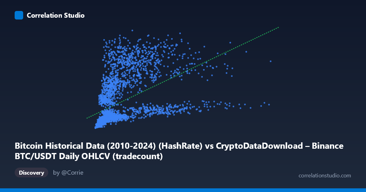
Bitcoin Historical Data (2010-2024) (HashRate) vs CryptoDataDownload – Binance BTC/USDT Daily OHLCV (tradecount)
- Pearson correlation (r)
- 0.4966
- Spearman correlation
- 0.7795
- p-value
- 0
- Sample size (n)
- 3191
- 95% confidence interval
- 0.47 to 0.5223
- Granger causality
- None
- Granger optimal lag
- 10
- Time coverage
- 2017-08-17 to 2026-05-20
AI analysis
Analysis: Bitcoin "HashRate" Column vs. Tradecount
Note on data labeling: the axis names appear mismatched with typical CDD conventions (a "HashRate" column and a "tradecount" column both sourced from BTC/USDT OHLCV data suggests these may actually represent volume-like and trade-count metrics rather than literal network hashrate). The analysis below treats them as the two numeric series provided, but this labeling ambiguity should be resolved before drawing domain-specific conclusions.
1. What the Visualization Reveals
The scatterplot shows a positive but noisy relationship: as X increases, Y tends to increase, but with substantial scatter at every level of X. The data is heavily right-skewed on both axes — X ranges from near-zero to over 15 million (mean ~1.97M, stdev ~2.24M, meaning stdev exceeds the mean), and Y spans from ~4M to ~1.3B. Most points cluster at low X values, with a long tail of large values pulling the range out. This skew is the classic signature of exchange trading data, where most days have modest activity punctuated by occasional extreme volume/activity days.
2. Strength, Direction, and Uncertainty
The Pearson correlation (r = 0.4966) indicates a moderate positive relationship, with r² = 0.2466 meaning only about 25% of the variance in Y is explained by X — leaving 75% driven by other factors or noise. The 95% CI [0.470, 0.522] is fairly tight given the large sample (n=3,191), and the p-value (~0) confirms the correlation is statistically robust and not due to chance — but statistical significance here reflects sample size more than practical strength. A moderate r² means X is a weak-to-moderate predictor of Y on its own.
The Granger causality tests are notable: neither direction shows significant predictive power (X→Y: p=0.48; Y→X: p=0.92) even at an optimal lag of 10 periods. This means neither series helps forecast the other's future values based on past values — the correlation is contemporaneous/associative, not predictive. Practically, this suggests both variables may be jointly driven by a third factor (e.g., overall market activity or price level) rather than one causing the other over time.
3. Notable Patterns and Non-linearity
The note that Spearman ρ exceeds Pearson r is important: it suggests the rank-order relationship is stronger than the linear one, pointing to a monotonic but curved relationship — likely logarithmic or power-law given the extreme skew in both variables. Small-X points show huge Y variability (e.g., X≈9,324 paired with Y≈7.6M, but X≈795,201 paired with Y≈947M), suggesting a compressed/saturating relationship at higher X, or that log-transforming both axes would linearize the pattern and likely raise the explained variance substantially. The residual scatter looks heteroscedastic — variance in Y grows with X, consistent with multiplicative rather than additive noise.
4. Confounding Factors and Caveats
Because both variables are derived from the same underlying BTC/USDT trading data, they likely share common drivers — price volatility, market-wide trading volume, and time trends (bull/bear cycles from 2017–2026) — creating spurious or mediated correlation rather than a direct causal link. Time itself is a hidden confound: if both series trend upward over the multi-year window (e.g., due to Bitcoin's growing adoption/exchange activity), correlating raw values without detrending can inflate r. The lack of Granger causality reinforces that this is likely a shared-trend/contemporaneous co-movement rather than a lead-lag causal mechanism.
5. Recommendations
- Log-transform both variables and re-run Pearson/regression — given the skew and Spearman Pearson gap, a log-log or log-linear model will likely fit much better and explain more variance. - Detrend or difference the series (e.g., first differences or year-over-year changes) to test whether the correlation survives after removing shared time trends — this addresses the confound directly. - Clarify column semantics — confirm whether "HashRate" and "tradecount" are correctly labeled, since both being sourced from OHLCV data is unusual for a hashrate metric. - Segment by market regime (bull/bear/sideways periods) to check if the relationship strength varies by volatility regime, which would explain some of the unexplained 75% variance. - Given no Granger causality, avoid using one series to forecast the other in isolation; consider a joint model with additional covariates (price, volatility, on-chain activity) instead.
X dataset: CryptoDataDownload – Binance BTC/USDT Daily OHLCV
Y dataset: Bitcoin Historical Data (2010-2024)
Part of experiment: Bitcoin - CryptoDataDownload – Binance BTC/USDT Daily OHLCV vs Bitcoin Historical Data (2010-2024)