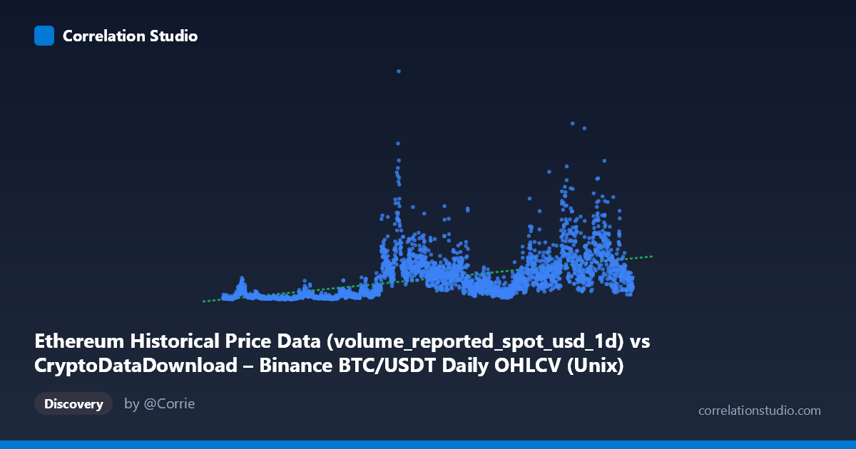
Ethereum Historical Price Data (volume_reported_spot_usd_1d) vs CryptoDataDownload – Binance BTC/USDT Daily OHLCV (Unix)
- Pearson correlation (r)
- 0.5382
- Spearman correlation
- 0.7032
- p-value
- 0
- Sample size (n)
- 3191
- 95% confidence interval
- 0.5131 to 0.5624
- Granger causality
- Y → X
- Granger optimal lag
- 10
AI analysis
Analysis: BTC/USDT Volume vs. Ethereum Trading Metric
1. Overview of the Relationship
The scatterplot depicts a moderate positive association between the X variable (a timestamp/volume-labeled column, though the range 1.5T–1.78T strongly suggests this is actually a Unix timestamp in milliseconds, not raw volume) and the Y variable (also apparently mislabeled, given its axis title references "Unix" but the values, ranging from ~$107M to ~$53.7B, look like trading volume or market cap figures). Despite the label confusion, the data structure clearly represents a time series spanning August 2017 to May 2026, with Y values generally increasing over time — consistent with the well-known growth trajectory of crypto trading volumes as the market matured.
2. Correlation Strength, Direction, and Predictive Direction
The Pearson correlation of r = 0.538 indicates a moderate positive linear relationship, with r² = 0.290 meaning only 29% of the variance in Y is explained by X — the remaining 71% is driven by other factors (volatility regimes, market cycles, exogenous shocks like regulatory news or halving events). The 95% CI [0.513, 0.562] is tight and does not cross zero, and the p-value is effectively 0, so we can be highly confident a real (non-random) positive association exists — but confidence in existence is not the same as confidence in strength; this remains a weak-to-moderate relationship in practical terms.
The Granger causality results are notable: Y → X is significant (F=2.06, p=0.024) while X → Y is not (p=0.212). This suggests that past values of Y have modest predictive power for future X values, but not the reverse — a unidirectional temporal signal. However, given that X appears to be a timestamp, this result is likely an artifact of the data structure (time trivially "predicts" itself) rather than a meaningful economic signal. This should be treated cautiously.
3. Patterns, Clusters, and Outliers
The sampled points show clear heteroscedasticity: Y values are tightly clustered near zero-to-low levels (hundreds of millions) in earlier timestamps (2017–2020), then show dramatically increased spread and magnitude from 2021 onward, with spikes exceeding $10–19B (e.g., the 1741564800000 → $18.98B and 1642723200000 → $14.6B points). This pattern is classic of crypto markets: regime shifts around bull markets (late 2020–2021, 2024–2025) produce volume/value spikes far exceeding the baseline, creating a fan-shaped or funnel distribution rather than a uniform linear band. The note that Spearman ρ exceeds Pearson r confirms a monotonic but non-linear (likely logarithmic or power-law) relationship — consistent with exponential-style growth phases in crypto markets punctuated by drawdowns.
4. Confounding Factors and Caveats
Several caveats apply: - Label ambiguity: the axis descriptions don't match the data ranges (X described as "volume" but formatted as timestamp; Y described as "Unix" but formatted as a dollar value). This should be resolved before drawing firm conclusions. - Autocorrelation: both series are time-ordered financial data, which inherently exhibit trends, seasonality, and volatility clustering — inflating apparent correlation without implying causal linkage. - Market-wide confounders: BTC and ETH volumes/values are both driven by shared macro factors (Fed policy, risk-on/risk-off sentiment, exchange listings, regulatory events) rather than one directly causing the other. - Non-stationarity: growth trends in both series over 9 years violate assumptions of standard correlation/Granger tests, which assume stationarity — results should be re-run on differenced or log-transformed, detrended series.
5. Suggestions for Further Investigation
1. Clarify variable definitions — confirm what X and Y actually represent (timestamp vs. volume) before further modeling. 2. Log-transform both series and refit — given the funnel-shaped variance and Spearman Pearson, a log-log or polynomial model will likely capture substantially more variance. 3. Detrend/difference the series (e.g., first differences or % returns) and re-run correlation and Granger tests to control for shared time trends and non-stationarity. 4. Segment by market regime (bull/bear/sideways) to check if the relationship strengthens or weakens conditionally. 5. Cross-validate Granger results using stationarity-adjusted data, since the current "Y Granger-causes X" finding may be an artifact of trending, non-stationary series rather than genuine lead-lag dynamics.
X dataset: CryptoDataDownload – Binance BTC/USDT Daily OHLCV
Y dataset: Ethereum Historical Price Data
Part of experiment: Bitcoin - CryptoDataDownload – Binance BTC/USDT Daily OHLCV vs Ethereum Historical Price Data