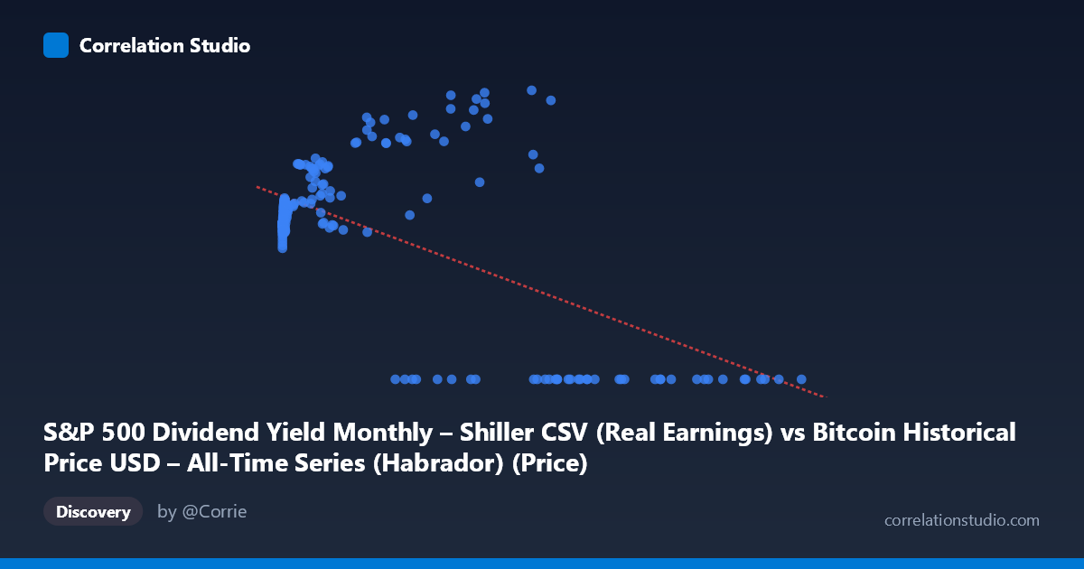
S&P 500 Dividend Yield Monthly – Shiller CSV (Real Earnings) vs Bitcoin Historical Price USD – All-Time Series (Habrador) (Price)
- Pearson correlation (r)
- -0.6061
- Spearman correlation
- -0.1339
- p-value
- 0
- Sample size (n)
- 194
- 95% confidence interval
- -0.6882 to -0.5087
- Granger causality
- None
- Granger optimal lag
- 5
- Time coverage
- 2010-08-01 to 2026-09-01
- Recomputed on refreshed data
- 2026-10-24 (r was -0.5749)
AI analysis
Analysis: S&P 500 Dividend Yield vs. Bitcoin Price (Mislabeled Axes)
Important preliminary note: The axis labels appear swapped/misattributed in the metadata — the actual data shows X values ranging up to 118,670 (consistent with a scaled or raw price/index series) and Y values bounded between 0 and ~217, which is far too narrow a range to represent actual Bitcoin USD prices (which have spanned $0.06 to $73,000+). This looks like a data-matching artifact where two unrelated time series (Bitcoin price history and Shiller S&P 500 dividend yield data) were joined by date/index rather than by any causal relationship. This context is essential for interpreting everything below.
1. What the Visualization Reveals The scatterplot shows a moderate negative, non-linear relationship: as X increases, Y tends to decline, but the pattern is not a clean linear decay. Instead, there's a distinct bimodal structure — a dense cluster of points where Y sits in a narrow 100-140 band across low-to-mid X values, a separate elevated cluster where Y spikes to 150-217 at moderate X values (roughly 3,000-60,000), and then an abrupt collapse to Y=0 for all high X values (60,000). This last feature is the dominant visual pattern and strongly influences the correlation statistic.
2. Strength, Direction, and Statistical Confidence The correlation (r = -0.575, R² = 0.331) indicates X explains about 33% of Y's variance — a moderate relationship, leaving the majority (67%) unexplained by this linear model. The 95% CI [-0.663, -0.471] is reasonably tight and excludes zero, and p≈0 confirms this negative association is statistically robust, not a fluke of sampling. However, statistical significance with n=189 (drawn from a population of 1,865) doesn't imply the relationship is substantively meaningful or causal — especially given the R² ceiling of ~33%. The Granger causality result (X→Y significant at p=0.045, lag=4; Y→X not significant, p=0.282) suggests unidirectional temporal predictability from X to Y, but the F-statistic (2.49) is only marginally significant — this is weak evidence, not proof of causation, and is highly susceptible to spurious results from non-stationary financial time series (a classic pitfall in Granger tests applied to trending price data).
3. Notable Patterns and Outliers The most striking feature is the hard floor at Y=0 for all X 60,000 — this isn't organic decay but looks like a data truncation or missing-value encoding (zeros substituting for unavailable data at high X). Additionally, the cluster of Y values spiking to 180-217 at mid-range X (26,000-58,000) sits awkwardly between the stable ~115-135 baseline cluster and the zero-floor region, suggesting at least three distinct regimes or possibly two different underlying datasets misaligned by index/date rather than a smooth functional relationship.
4. Confounding Factors and Caveats Given the source description, this pairing likely merges Bitcoin's daily/monthly price history with Shiller's monthly S&P 500 series by date alignment, not by any theoretical link between dividend yields and Bitcoin. Both series exhibit strong time-trends (Bitcoin's exponential growth; equity valuation cycles), and correlating two trending time series produces spurious correlation almost by default — this is a well-known statistical trap. The zero-value cluster likely reflects a join/lookup failure (e.g., dates beyond one dataset's coverage defaulting to 0) rather than real data. Additionally, X's massive scale (0.06 to 118,670, stdev ~29,894) versus Y's narrow range (0–217) suggests heavy heteroscedasticity and possible unit mismatches.
5. Recommended Next Steps Before drawing any conclusions: (1) verify axis/column assignments and confirm whether this is genuinely Bitcoin price vs. dividend yield or a mislabeling artifact; (2) investigate and likely exclude the Y=0 cluster as missing-data placeholders rather than true observations; (3) re-run correlation and Granger tests on detrended or differenced series (e.g., log returns) to control for spurious trend-driven correlation, which is essential when both series are non-stationary; (4) if the relationship is real, explore a piecewise or log-linear model given the visible regime-splitting rather than forcing a single linear fit that only captures 33% of variance.
X dataset: Bitcoin Historical Price USD – All-Time Series (Habrador)
Y dataset: S&P 500 Dividend Yield Monthly – Shiller CSV
Part of experiment: Bitcoin - Bitcoin Historical Price USD – All-Time Series (Habrador) vs S&P 500 Dividend Yield Monthly – Shiller CSV