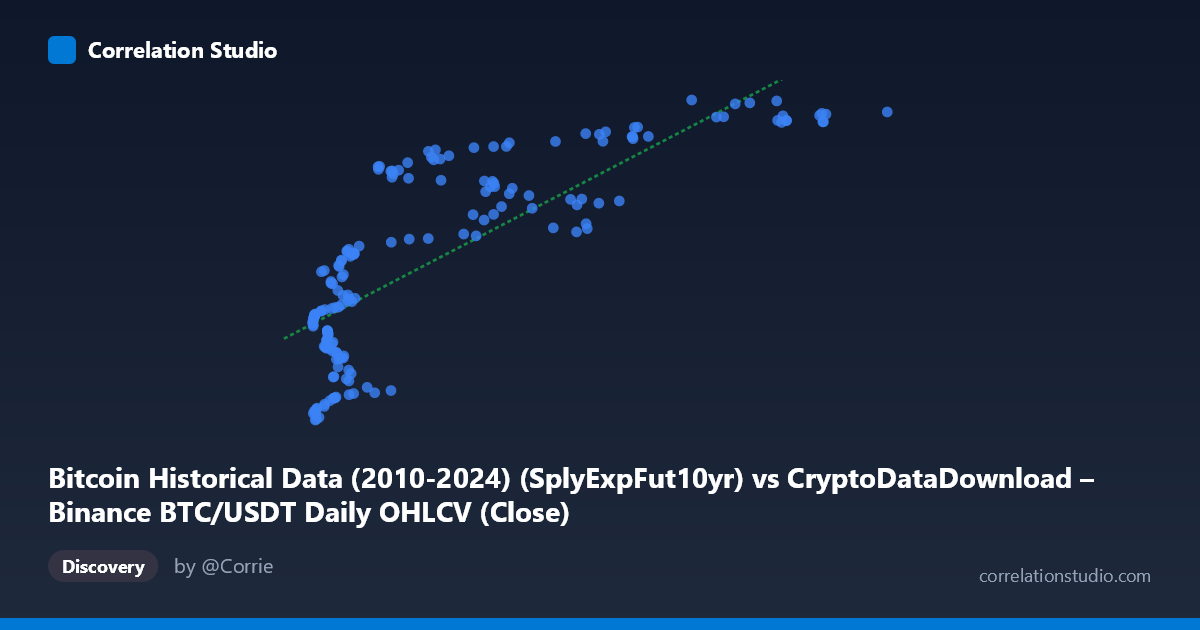
Bitcoin Historical Data (2010-2024) (SplyExpFut10yr) vs CryptoDataDownload – Binance BTC/USDT Daily OHLCV (Close)

Pearson correlation (r): 0.8021
Spearman correlation: 0.8265
p-value: 0
Sample size (n): 180
95% confidence interval: 0.7429 to 0.8488
Granger causality: None
Granger optimal lag: 10

AI analysis

Analysis: Bitcoin Supply Metric vs. BTC/USDT Closing Price

1. Relationship Overview

The scatterplot depicts a positive, moderately-strong association between a Bitcoin supply-based metric ("SplyExpFut10yr" — likely a projected/expected future supply calculation) and the BTC/USDT daily closing price. The data shows a clear upward-sloping pattern, but it is distinctly non-linear/curved rather than a clean straight line — the relationship appears to flatten out at higher X values, suggesting a logarithmic or saturating curve rather than a strictly linear one, even though the linear fit captures a reasonable share of the variance.

2. Strength, Direction, and Predictive Uncertainty

The correlation (r = 0.80, r² = 0.643) indicates that roughly 64% of the variance in Y (closing price) is statistically associated with variance in X, leaving ~36% explained by other factors or noise. The 95% CI [0.743, 0.849] is reasonably tight given n=180, and the p-value of ~0 confirms this correlation is highly unlikely to be due to chance in-sample. However, "highly significant" here refers to statistical significance, not necessarily causal strength — with r² at 0.64, this is a good but incomplete predictor relationship, not a near-deterministic one.

Critically, the Granger causality tests show no significant predictive direction in either direction (X→Y: p=0.43; Y→X: p=0.64) at the optimal lag of 10 periods. This is an important caveat: despite the strong contemporaneous correlation, neither series helps forecast the other's future values beyond what its own past values provide. This strongly suggests the relationship is not a simple lead-lag mechanism but more likely reflects a shared underlying driver — both variables are probably deterministic or near-deterministic functions of the same clock/blockchain state (e.g., block height, elapsed time, or halving schedule), meaning they co-move because they're both proxies for "time" or "network maturity" rather than one causing the other.

3. Notable Patterns and Clusters

The data shows distinct clustering rather than a smooth continuum: - A dense cluster at low X (3,700–20,000) with Y ranging widely (20.2M–20.7M), indicating high price variability at low X values — this is where most of the noise/scatter lives. - A tighter, more linear-looking cluster at high X (60,000–105,000) where Y compresses into a narrow band (20.75M–20.83M), suggesting saturation. - A visible "elbow" or inflection around X ≈ 20,000–40,000, consistent with a logarithmic curve (e.g., Y ~ a·ln(X) + b) rather than the linear fit reported. This would explain why residuals are likely heteroscedastic — larger scatter at low X, tighter fit at high X.

4. Confounding Factors and Caveats

- Autocorrelation/non-independence: Both series are time-series with a 2017–2026 span; daily financial and supply-derived data are highly autocorrelated, meaning the "n=180" effective sample size is likely overstated for standard significance testing (both variables trend with time, inflating r without necessarily reflecting a true bivariate relationship). - Shared time trend: Since Bitcoin's supply schedule is fully deterministic and price generally trended upward over this period, much of the correlation may simply reflect that both are monotonic functions of calendar time — a classic spurious-correlation setup unless detrended. - Non-linearity mischaracterized by linear r²: The apparent curve shape means the reported linear R²=0.643 likely understates the true relationship strength; a log or power transform of X could yield a notably better fit. - Sampling: n=180 is drawn from a population of 3,212 — every 3rd point per the summary — so ensure this systematic sampling didn't introduce periodicity bias.

5. Suggested Next Steps

- Re-run the correlation on detrended or differenced series (e.g., % daily returns/changes) to test whether the relationship holds beyond shared time-trend, which would give a more causally meaningful picture. - Test a log-linear or logistic model (Y vs. ln(X)) given the visual saturation pattern — likely a materially better fit than the linear model. - Given null Granger causality, avoid using this metric as a short-term price predictor; instead treat both as co-integrated long-run indicators tied to Bitcoin's issuance/maturity cycle — a cointegration test (e.g., Engle-Granger) would be more appropriate than Granger causality on levels. - Segment analysis by halving-cycle era, since supply-based metrics behave discretely around halving events, which may explain the clustering/elbow pattern.

X dataset: CryptoDataDownload – Binance BTC/USDT Daily OHLCV

Y dataset: Bitcoin Historical Data (2010-2024)

Part of experiment: Bitcoin - CryptoDataDownload – Binance BTC/USDT Daily OHLCV vs Bitcoin Historical Data (2010-2024)