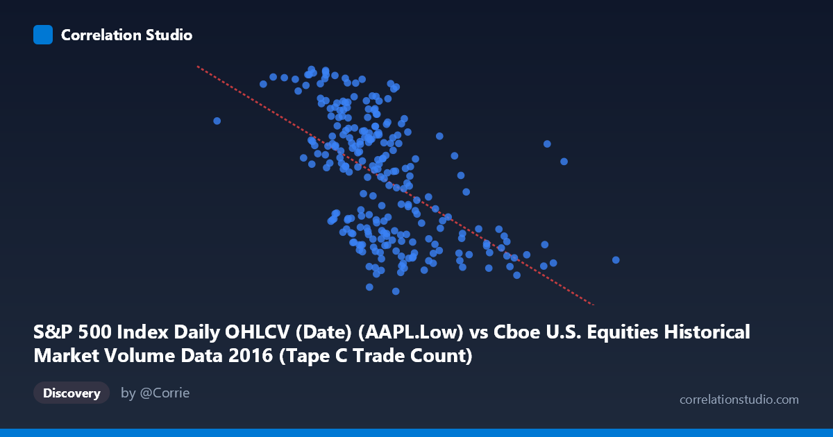
S&P 500 Index Daily OHLCV (Date) (AAPL.Low) vs Cboe U.S. Equities Historical Market Volume Data 2016 (Tape C Trade Count)
- Pearson correlation (r)
- -0.5527
- Spearman correlation
- -0.585
- p-value
- 0
- Sample size (n)
- 252
- 95% confidence interval
- -0.633 to -0.4606
- Granger causality
- None
- Granger optimal lag
- 1
AI analysis
Analysis: AAPL Low Price vs. Cboe Tape C Trade Count (2016)
Relationship Overview The scatterplot reveals a moderate negative relationship between Apple's daily low price (X-axis) and the Cboe Tape C trade count (Y-axis) over 2016. As AAPL's low price increases, the number of trades on Cboe's Tape C exchange tends to decrease. The linear regression equation (y = -2.90312E-05x + 124.4) confirms this inverse slope, suggesting that for every ~34,000-point increase in AAPL's low price, Tape C trade count decreases by approximately one unit. The data spans a wide X-range (~277K to ~1.32M) with Y values clustered between roughly 89 and 117, indicating that trade count variation is relatively constrained compared to the broad price range observed.
Correlation Strength and Statistical Significance The Pearson correlation of r = -0.5527 indicates a moderate negative association, and the R² of 0.3055 means that approximately 30.5% of the variance in Tape C trade count is explained by AAPL's low price — leaving nearly 70% attributable to other factors. The 95% confidence interval of [-0.6330, -0.4606] is entirely negative and reasonably tight, providing strong evidence that the true population correlation is meaningfully negative rather than a sampling artifact. The p-value of effectively zero confirms high statistical significance given n=252 paired observations. However, despite statistical significance, the Granger causality tests are non-significant in both directions (X→Y: F=1.33, p=0.249; Y→X: F=0.98, p=0.324), indicating that neither variable temporally predicts the other at a 1-period lag. This is a critical caveat: the correlation reflects a contemporaneous co-movement, not a predictive or causal temporal relationship.
Notable Patterns and Outliers The sample points reveal considerable scatter around the regression line, consistent with an R² of ~0.31. Several notable features emerge: a cluster of points in the 600K–750K X-range showing wide Y dispersion (89–116), suggesting that at mid-range AAPL prices, trade count is highly variable. Points such as (746,425, 89.47) and (519,409, 116.78) represent near-extremes on both axes simultaneously, reinforcing the negative trend. At the higher X-range (e.g., 990,202 at Y=92.39; 1,023,027 at Y=94.94), trade counts are consistently low, forming a tighter cluster that anchors the negative slope. The lower-left region is sparsely populated, suggesting AAPL rarely traded at very low prices during 2016, which aligns with Apple's general price appreciation that year.
Confounding Factors and Caveats Several important caveats apply. First, the axis labels appear potentially swapped in the metadata — AAPL Low is listed as X but sourced from the Cboe dataset, and Tape C Trade Count is sourced from the S&P 500 OHLCV dataset, suggesting possible dataset join or labeling inconsistencies that warrant verification. Second, both variables are time-indexed to 2016, meaning shared macroeconomic drivers (e.g., market volatility events, FOMC decisions, Brexit) could simultaneously move both series, creating spurious correlation. Third, AAPL's price trajectory in 2016 (generally recovering from early-year lows) introduces temporal autocorrelation that may inflate the apparent cross-sectional relationship. Fourth, Tape C specifically covers NYSE-listed securities, so its trade count reflects broad market activity beyond just AAPL, making a direct causal narrative tenuous.
Actionable Insights and Further Investigation Given the moderate correlation without Granger causality, this relationship is best interpreted as coincidental co-movement driven by shared market conditions rather than any direct link. Practitioners should: (1) partial out market-wide volatility (e.g., VIX) and overall volume to test whether the residual correlation persists; (2) extend lag testing beyond 1 period in Granger analysis, as market effects sometimes manifest over 3–5 trading days; (3) segment the data by market regime (high vs. low volatility periods) to determine whether the correlation strengthens during stress events; and (4) verify dataset join integrity, ensuring X and Y values are correctly aligned by date before drawing further conclusions. A rolling-window correlation analysis across 2016 quarters could also reveal whether this relationship was stable or concentrated in specific periods.
X dataset: Cboe U.S. Equities Historical Market Volume Data 2016
Y dataset: S&P 500 Index Daily OHLCV (Date)
Part of experiment: Daily - Cboe U.S. Equities Historical Market Volume Data 2016 vs S&P 500 Index Daily OHLCV (Date)