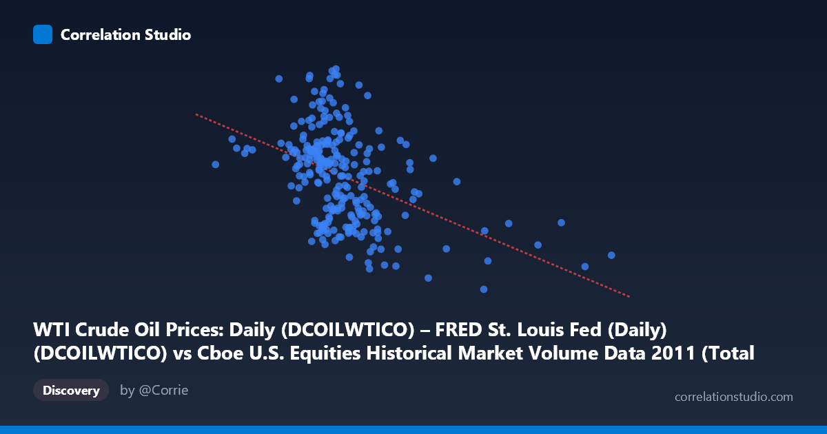
WTI Crude Oil Prices: Daily (DCOILWTICO) – FRED St. Louis Fed (Daily) (DCOILWTICO) vs Cboe U.S. Equities Historical Market Volume Data 2011 (Total Shares)
- Pearson correlation (r)
- -0.4384
- Spearman correlation
- -0.4479
- p-value
- 0
- Sample size (n)
- 252
- 95% confidence interval
- -0.5331 to -0.3328
- Granger causality
- None
- Granger optimal lag
- 1
AI analysis
Analysis: WTI Crude Oil Prices vs. U.S. Equity Market Volume (2011)
Relationship Overview The scatterplot reveals a moderate negative relationship between WTI crude oil prices (X-axis) and total U.S. equity market shares traded (Y-axis) across 252 trading days in 2011. The linear regression equation (y = -2.88×10⁻⁸x + 109.935) captures a downward-sloping trend: as oil prices rise, equity trading volume tends to decline. This pattern is economically intuitive — higher oil prices can dampen investor risk appetite, increase uncertainty, and reduce speculative equity activity. However, the scatter around the regression line is considerable, suggesting this relationship is real but far from deterministic.
Correlation Strength and Statistical Significance The Pearson correlation of r = -0.4384 indicates a moderate negative association, but the variance explained metric is the more sobering figure: R² = 0.1922, meaning oil prices account for only about 19.2% of the variance in equity trading volume. Roughly 80% of what drives daily volume fluctuations lies elsewhere. The 95% confidence interval of [-0.5331, -0.3328] is entirely negative, confirming directional consistency, and the p-value of 2.944×10⁻¹³ — derived from a population of N = 3,780 — makes it statistically implausible that this correlation is a chance artifact. That said, statistical significance here is partially a function of large sample size; the practical effect size remains modest. Granger causality results complicate the story further: neither direction shows significant temporal predictability at conventional thresholds (X→Y: F = 0.115, p = 0.734; Y→X: F = 3.753, p = 0.054). Oil prices do not reliably predict next-day equity volume, nor does volume predict oil prices, suggesting the observed correlation reflects contemporaneous co-movement rather than a lead-lag causal mechanism.
Patterns, Clusters, and Outliers Several notable features emerge from the sample points. The bulk of observations cluster in the oil price range of $450M–$650M (roughly $85–$110/barrel equivalent range on the X axis) with volume between 85 and 108, forming a moderately dense core. There are visible outliers at the high end of X — points near $800M–$878M oil price values that show relatively low volume (~85–94), consistent with the negative trend. Conversely, a cluster at lower oil prices (e.g., ~$242M–$360M range) shows elevated or average volume (~100–112), reinforcing the negative slope. The point at approximately (360M, 111.68) stands out as a high-volume, low-price observation that strongly influences the regression. The distribution also appears heteroscedastic — variance in volume seems wider at mid-range oil prices and somewhat compressed at extremes — which warrants caution about the uniform assumptions of OLS regression.
Confounding Factors and Caveats Several confounds could explain or distort this correlation. 2011 was a particularly volatile year — encompassing the Eurozone debt crisis, U.S. debt ceiling debate, Arab Spring disruptions to oil supply, and the August 2011 market crash — meaning both variables were simultaneously responding to common macro shocks rather than causally influencing each other. This is a classic spurious correlation via common driver scenario. Additionally, equity trading volume is influenced by VIX (volatility), algorithmic trading activity, earnings seasons, and Federal Reserve communications, none of which are controlled here. The dataset labels also appear swapped in the axis descriptions (the notes describe each variable as belonging to the other dataset), which should be verified before drawing firm conclusions. Finally, using daily data without accounting for autocorrelation or time-series structure in either variable may inflate the effective sample size and therefore the apparent significance.
Actionable Insights and Further Investigation Given the modest explanatory power and absent Granger causality, practitioners should not use oil prices as a standalone predictor of equity volume. However, the consistent negative correlation warrants inclusion of oil price changes as a control variable in broader volume-forecasting models. Further investigation should: (1) decompose the time series using rolling-window correlations to test whether the relationship strengthened during specific 2011 stress episodes; (2) introduce VIX and macro surprise indices as covariates to test whether the oil-volume relationship survives controls; (3) examine whether the relationship holds at sector level (e.g., energy stocks vs. tech stocks may show opposite volume responses to oil); and (4) extend the analysis across multiple years to determine whether 2011's correlation is year-specific or structurally persistent. A regime-switching or quantile regression approach may also better capture the non-linear, heteroscedastic features visible in the scatterplot.
X dataset: Cboe U.S. Equities Historical Market Volume Data 2011
Y dataset: WTI Crude Oil Prices: Daily (DCOILWTICO) – FRED St. Louis Fed (Daily)
Part of experiment: Daily - Cboe U.S. Equities Historical Market Volume Data 2011 vs WTI Crude Oil Prices: Daily (DCOILWTICO) – FRED St. Louis Fed (Daily)