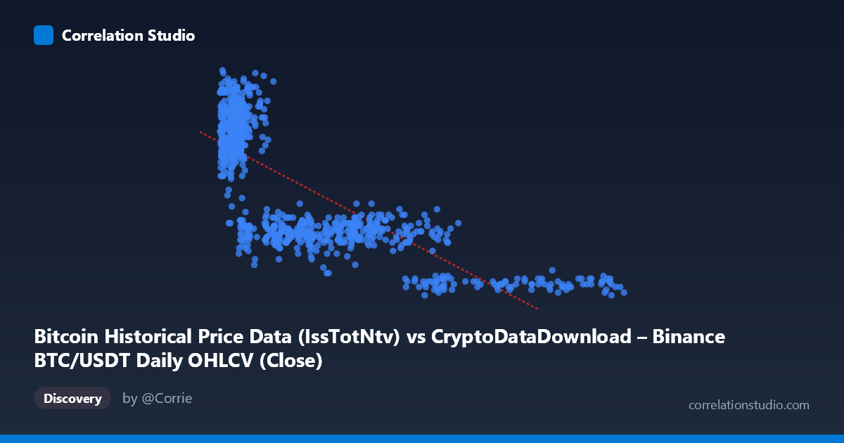
Bitcoin Historical Price Data (IssTotNtv) vs CryptoDataDownload – Binance BTC/USDT Daily OHLCV (Close)

Pearson correlation (r): -0.7761
Spearman correlation: -0.7616
p-value: 0
Sample size (n): 938
95% confidence interval: -0.8004 to -0.7494
Granger causality: None
Granger optimal lag: 10
Time coverage: 2017-08-20 to 2026-05-20

AI analysis

Analysis: BTC "IssTotNtv" vs. BTC/USDT Close Price

1. What the Visualization Reveals

The scatterplot shows a clear inverse, curvilinear relationship between the X variable (labeled as Bitcoin's total issued native units, IssTotNtv) and Y (BTC/USDT closing price). As X increases from roughly 3,000 to over 120,000, Y systematically declines from highs near 2,000–2,375 down to below 500. The data points cluster densely at low X values (under 15,000) with high, variable Y values (1,600–2,225), then thin out and flatten toward low Y values as X grows into the tens of thousands and beyond. This pattern is consistent with a decaying/inverse function shape rather than a straight line, despite the linear model fitting reasonably well.

2. Strength, Direction, and Predictive Relationship

The correlation coefficient (r = -0.776) indicates a strong negative linear association, with r² = 0.602 meaning approximately 60% of the variance in Y is statistically explained by X — a substantial but not complete relationship, leaving ~40% driven by other factors or noise. The tight 95% CI [-0.800, -0.749] and p-value of 0 confirm this correlation is highly statistically robust and not a product of sampling noise, especially given the large sample (n=938). However, the Granger causality tests reveal an important caveat: neither variable significantly predicts the other over time (X→Y: p=0.306; Y→X: p=0.719). This means that despite the strong contemporaneous correlation, there's no evidence of a lagged, directional, predictive relationship — the two series move together but not in a way where past values of one forecast future values of the other at the tested lag structure (10 periods).

3. Notable Patterns and Non-Linear Features

The most striking feature is the curvature: Y drops steeply as X increases from 3,000 to ~30,000, then the decline decelerates, with Y asymptotically approaching low values (400–500) as X exceeds 60,000–120,000. This suggests a power-law, logarithmic, or inverse relationship might fit better than a straight line. There's also a dense cluster of points at low X (3,000–15,000) with high Y variance, suggesting either heteroscedasticity or a secondary factor influencing Y in that region. No extreme outliers are apparent, but the sparse, spread-out points at high X (e.g., 98,000–121,000) carry disproportionate leverage on the linear regression fit.

4. Confounding Factors and Caveats

Both variables are derived from Bitcoin market/network data over a multi-year period (2017–2026) spanning multiple bull/bear cycles, halving events, and macroeconomic regimes (e.g., 2017 mania, 2020-21 bull run, 2022 crash). Time itself is a major latent confounder — both series may be independently trending due to broader adoption, regulatory shifts, or market cycles, producing spurious correlation without causal linkage. Additionally, if "IssTotNtv" reflects total issued supply or a cumulative/monotonically increasing network metric, it will naturally trend with time, while price is non-monotonic and cyclical — meaning the negative correlation could be an artifact of comparing a secular trend against a cyclical price series rather than a true economic mechanism.

5. Actionable Insights and Further Investigation

Given the non-linear pattern, fitting a log-linear, power, or exponential decay model (e.g., regressing log(Y) on X or log(X)) would likely improve explanatory power beyond the current 60.2% R². Since Granger tests show no predictive causality, this relationship should not be used for forecasting one variable from the other; instead, treat it as a descriptive/structural association possibly driven by shared time trends or halving-driven supply dynamics. Further work should include: (a) detrending both series or analyzing returns/changes instead of levels to test for spurious correlation, (b) segmenting the data by market cycle/halving epoch to see if the relationship is stable or regime-dependent, and (c) incorporating additional covariates (e.g., trading volume, macro liquidity indices) to isolate whether X truly has explanatory power over Y or both are proxies for a common underlying driver (time/adoption).

X dataset: CryptoDataDownload – Binance BTC/USDT Daily OHLCV

Y dataset: Bitcoin Historical Price Data

Part of experiment: Bitcoin - CryptoDataDownload – Binance BTC/USDT Daily OHLCV vs Bitcoin Historical Price Data