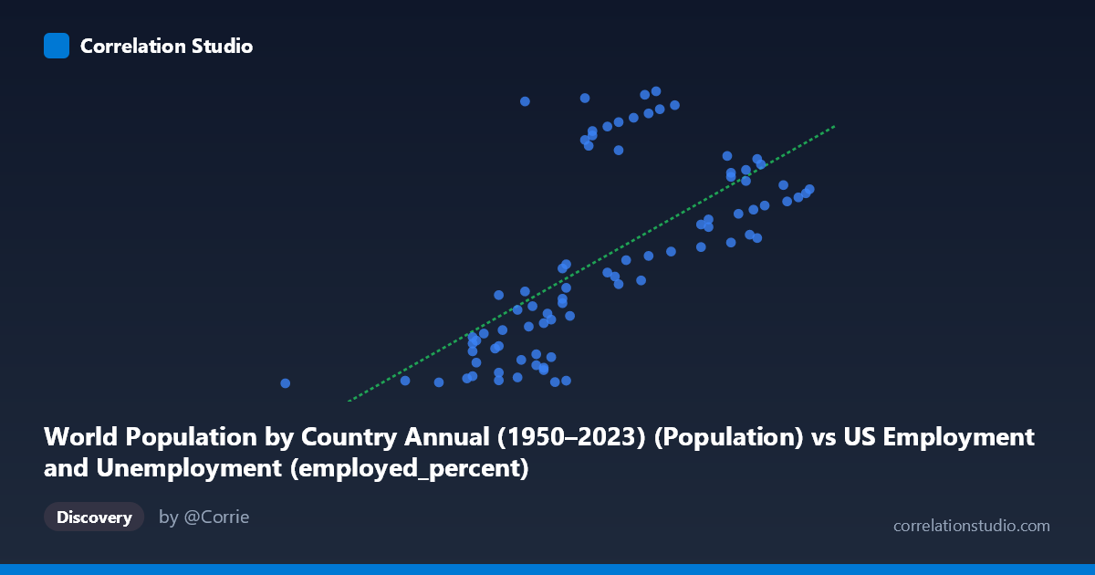
World Population by Country Annual (1950–2023) (Population) vs US Employment and Unemployment (employed_percent)
- Pearson correlation (r)
- 0.6689
- Spearman correlation
- 0.7328
- p-value
- 0
- Sample size (n)
- 83
- 95% confidence interval
- 0.5296 to 0.773
- Granger causality
- None
- Granger optimal lag
- 10
- Time coverage
- 1941-01-01 to 2023-01-01
AI analysis
Scatterplot Analysis: World Population vs. US Employment Percentage
Overview of the Relationship
The scatterplot reveals a moderate positive relationship between world population (X-axis, ranging roughly 50–64 in units consistent with the dataset's population scaling) and the US employed percentage (Y-axis, ranging from approximately 46 million to 163 million). As world population increases, US employment figures tend to rise as well. The linear regression equation (y = 8,488,420x − 403,097,000) captures this upward trend, though considerable scatter around the regression line is immediately apparent, suggesting the relationship is far from deterministic. The time coverage of 1941–2023 means both variables are fundamentally time-driven series, which is a critical interpretive caveat.
Correlation Strength and Statistical Significance
The Pearson correlation of r = 0.6689 indicates a moderate-to-strong positive association, but the explanatory power is more sobering: r² = 0.4474 means that only ~44.7% of the variance in US employment percentage is statistically explained by world population, leaving over 55% attributable to other factors. The 95% confidence interval for r of [0.530, 0.773] is reasonably tight and does not include zero, and the p-value of 4.82×10⁻¹² confirms this correlation is highly statistically significant given n = 83 paired observations. However, statistical significance here almost certainly reflects the shared upward trend of both variables over time (a classic spurious correlation problem) rather than any genuine causal mechanism. Crucially, Granger causality testing finds no significant directional predictive relationship in either direction — neither X→Y (F = 1.11, p = 0.37) nor Y→X (F = 1.61, p = 0.13) — meaning neither variable meaningfully predicts the other temporally after accounting for their own past values. This is a strong signal that the correlation is likely coincidental trend co-movement.
Notable Patterns, Clusters, and Outliers
Several features stand out in the data. There is a visible cluster of points in the lower-left region (X ≈ 50–57, Y ≈ 46–85 million), likely corresponding to earlier decades (1940s–1970s) when both world population and US employment were lower. A second cluster emerges in the upper-right (X ≈ 60–64, Y ≈ 100–165 million), corresponding to more recent decades. Notably, vertical spread within narrow X-bands is extremely wide — for example, at X ≈ 56–58, Y values range from ~47 million to over 159 million (e.g., the point at 56.80 recording 159,152,462 appears far above its neighbors). Similarly, points like (60.30, 163,211,907) and (60.00, 161,811,336) sit dramatically above the regression line, while (50.40, 46,410,179) anchors the lower extreme. These high-leverage outliers suggest that year-specific economic shocks — recessions, post-war booms, or labor force structural changes — dominate variation that population cannot explain.
Confounding Factors and Interpretive Caveats
This correlation almost certainly reflects spurious co-trending rather than a meaningful causal link. Both world population and US employment have grown steadily over the 1941–2023 period due to entirely independent forces: global demographic momentum on one hand, and US labor force expansion, immigration, women entering the workforce, and economic growth on the other. Any two variables that trend upward over the same historical window will correlate positively without implying causation. Additionally, the dataset column assignments appear counterintuitive — "employedpercent" is labeled as coming from the population dataset, and "Population" from the employment dataset — suggesting possible metadata misalignment that warrants verification. The wide within-cluster scatter also hints at non-linearity or regime changes (e.g., WWII mobilization, 2008 financial crisis, COVID-19) that a simple linear model cannot capture.
Actionable Insights and Further Investigation
Given the absence of Granger causality and the likely spurious nature of the correlation, practitioners should avoid using world population as a predictor of US employment in any applied forecasting model. Recommended next steps include: (1) detrending both series (e.g., first-differencing or HP filtering) before re-examining correlation to isolate cyclical from trend variation; (2) verifying the dataset column mappings, as the axis descriptions suggest the variables may have been swapped between datasets; (3) investigating the high-residual outlier years to understand what economic events drove extreme deviations; and (4) introducing economically meaningful covariates — GDP growth, participation rate changes, or policy variables — in a multivariate framework to properly attribute variance in US employment figures.
X dataset: US Employment and Unemployment
Y dataset: World Population by Country Annual (1950–2023)
Part of experiment: Yearly - US Employment and Unemployment vs World Population by Country Annual (1950–2023)