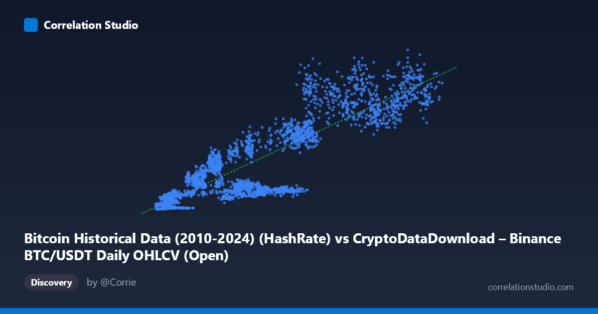
Bitcoin Historical Data (2010-2024) (HashRate) vs CryptoDataDownload – Binance BTC/USDT Daily OHLCV (Open)
- Pearson correlation (r)
- 0.891
- Spearman correlation
- 0.8818
- p-value
- 0
- Sample size (n)
- 3191
- 95% confidence interval
- 0.8837 to 0.898
- Granger causality
- None
- Granger optimal lag
- 10
AI analysis
Analysis: Bitcoin Hash Rate vs. Opening Price
1. What the Visualization Reveals
The scatterplot shows a clear positive, non-linear relationship between Bitcoin's hash rate (X) and its opening price (Y). Data points sweep from a dense cluster of low-value observations (hash rate < 15,000, price < $150M) through a widening spray of high-value points (hash rate 80,000, price approaching $1.3B). The pattern resembles a curved fan shape rather than a tight linear band — variance in Y increases substantially as X increases, a classic sign of heteroscedasticity.
2. Strength, Direction, and Uncertainty
The correlation coefficient (r = 0.891) indicates a strong positive linear relationship, with r² = 0.794 meaning roughly 79% of the variance in price is statistically associated with variance in hash rate. The tight 95% confidence interval [0.884, 0.898] combined with p ≈ 0 confirms this correlation is highly stable and not a product of sampling noise, given the large sample size (n = 3,191). However, correlation here does not imply prediction: the Granger causality tests show neither variable significantly predicts the other at the tested lag structure (X→Y: p = 0.473; Y→X: p = 0.136). This is a critical distinction — the two series move together over the long run (likely both trending upward over 2017–2026), but neither's past values offer meaningful forecasting power over the other's future values in this framework.
3. Notable Patterns and Outliers
Several features stand out: - Fan/cone shape: At low hash rates (< 10,000), prices are tightly clustered near the bottom (under $50M), but as hash rate rises above 60,000–80,000, the spread in price balloons dramatically (from ~$150M to over $1.1B for similar X values). This suggests the relationship may be better modeled as exponential/power-law rather than linear. - Inconsistent pairs: Points like (57,635 → $158M) sit far below others with similar hash rate (57,037 → $605M), indicating hash rate alone doesn't tightly pin down price at any given level — other factors (market cycles, sentiment) dominate at mid-range values. - No visible clusters or regime breaks are obvious from the sample, but the widening variance suggests at least two behavioral regimes: an early low-hash-rate/low-price era and a later high-hash-rate/high-price era with much more volatility.
4. Confounding Factors and Caveats
- Shared time trend: Both hash rate and price have risen secularly over the 2017–2026 window (mining infrastructure growth alongside adoption/appreciation). This is a classic case where two unrelated-but-trending time series can show strong correlation without direct causal linkage — a well-known spurious correlation risk in time series analysis. - Reverse mechanics: Economically, rising price incentivizes more mining investment (raising hash rate), while hash rate itself does not directly set price — it reflects mining economics/difficulty. The Granger results (no significant predictive direction either way at this lag) are consistent with both variables responding to a common latent driver (e.g., overall market cycle) rather than one causing the other. - Non-stationarity: Both series likely have unit roots (trending, non-stationary), which inflates r² artificially in raw-level regressions. Standard OLS/correlation may overstate the "true" relationship. - Heteroscedasticity: The fan-shaped variance violates the constant-variance assumption in the linear regression, making the R²=0.794 estimate less trustworthy for inference (though fine descriptively).
5. Suggested Next Steps
1. Detrend/difference the series (e.g., use % daily returns or first differences) and re-run correlation and Granger tests — this will reveal whether the relationship holds beyond the shared upward trend. 2. Log-transform both variables given the apparent multiplicative/exponential scaling, then refit — a log-log model likely fits the fan-shaped data better than the current linear form. 3. Test cointegration (e.g., Johansen or Engle-Granger) to see if hash rate and price share a long-run equilibrium relationship despite each being non-stationary individually. 4. Segment by market era/halving cycle to check if the relationship strength or slope changes across bull/bear regimes. 5. Treat hash rate as a lagging indicator of mining profitability, not a leading price signal, and explore other candidate predictors (transaction volume, active addresses, macro liquidity conditions) for genuine forecasting utility.
X dataset: CryptoDataDownload – Binance BTC/USDT Daily OHLCV
Y dataset: Bitcoin Historical Data (2010-2024)
Part of experiment: Bitcoin - CryptoDataDownload – Binance BTC/USDT Daily OHLCV vs Bitcoin Historical Data (2010-2024)