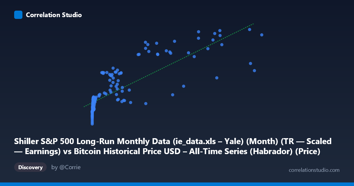
Shiller S&P 500 Long-Run Monthly Data (ie_data.xls – Yale) (Month) (TR — Scaled — Earnings) vs Bitcoin Historical Price USD – All-Time Series (Habrador) (Price)
- Pearson correlation (r)
- 0.8124
- Spearman correlation
- 0.9088
- p-value
- 0
- Sample size (n)
- 155
- 95% confidence interval
- 0.7509 to 0.8599
- Granger causality
- None
- Granger optimal lag
- 10
AI analysis
Analysis: Bitcoin Price vs. Shiller S&P 500 Earnings-Scaled Data
1. What the Visualization Reveals
The scatterplot shows a positive, moderately strong relationship between the Shiller S&P 500 earnings-related metric (X-axis) and Bitcoin's historical USD price (Y-axis). As X increases from near-zero values into the tens of thousands, Y rises from roughly $52,000–$62,000 up toward $130,000+. The data forms a curved, fan-shaped pattern rather than a tight linear band—dense clustering at low X values (under ~15,000) with wider dispersion at higher X values, suggesting the relationship may be better described as log-linear or concave rather than strictly linear.
2. Strength, Direction, and Predictive Relationship
The correlation coefficient (r = 0.81) indicates a strong positive linear association, with R² = 0.66 meaning the linear model explains 66% of the variance in Y—substantial, but leaving roughly a third of variability unexplained. The 95% CI [0.75, 0.86] is fairly tight given n=155, and the p-value (effectively 0) confirms this correlation is highly unlikely due to chance. However, the Granger causality tests are critical here: neither direction (X→Y or Y→X) shows statistical significance (p = 0.60 and p = 0.77, respectively) even at an optimal lag of 10 periods. This means despite the strong contemporaneous correlation, neither series meaningfully predicts the other's future movements—the relationship is associative, not temporally causal or predictive in a forecasting sense.
3. Notable Patterns and Outliers
Several features stand out: a dense cluster of low-X points (X < 1,000) with Y values ranging widely from ~$52,000 to ~$99,000, indicating high variance in Bitcoin price when the Shiller metric is near zero—likely reflecting Bitcoin's early years (low/no correlation to traditional equity earnings metrics). A notable outlier appears at (45,092.81, 93,913.81), which sits well below the regression line compared to neighboring points like (43,718, 129,334) and (46,208, 138,102)—this could represent a Bitcoin bear-market trough coinciding with elevated Shiller values. The overall shape hints at nonlinearity: Bitcoin's price growth appears to decelerate or plateau at the highest X values (60,000+), rather than continuing linearly.
4. Confounding Factors and Caveats
This is almost certainly a spurious or coincidental correlation driven by shared time trends rather than any economic mechanism linking Shiller's earnings-scaled equity metric to Bitcoin prices. Both series have grown substantially over the 2010–2023 window (Bitcoin due to adoption/speculation, the Shiller metric due to long-run equity market appreciation), so the correlation may simply reflect two independent upward trends over time (a classic "time as confound" issue). The lack of Granger causality strongly supports this interpretation—if the relationship were causal, we'd expect at least weak lead-lag predictive power. Additionally, mismatched sampling frequencies (monthly Shiller data vs. Bitcoin's continuous price series) and the vastly different economic domains (equity market earnings vs. a speculative digital asset) make a direct causal link implausible.
5. Actionable Insights and Further Investigation
Given the Granger results, this correlation should not be used for trading or forecasting purposes—it offers no predictive edge in either direction. To properly assess whether this is spurious, analysts should: (a) detrend both series (e.g., via differencing or log-returns) and re-test correlation/causality on stationary data, since raw trending series often produce inflated correlations; (b) test against a common confounding factor, such as overall macro liquidity (M2 money supply, real interest rates, or time itself) which may drive both series independently; and (c) explore nonlinear/log-log transformations given the fan-shaped, non-uniform variance pattern, which may better characterize the true functional relationship if one exists.
X dataset: Bitcoin Historical Price USD – All-Time Series (Habrador)
Y dataset: Shiller S&P 500 Long-Run Monthly Data (ie_data.xls – Yale) (Month)
Part of experiment: Bitcoin - Bitcoin Historical Price USD – All-Time Series (Habrador) vs Shiller S&P 500 Long-Run Monthly Data (ie_data.xls – Yale) (Month)