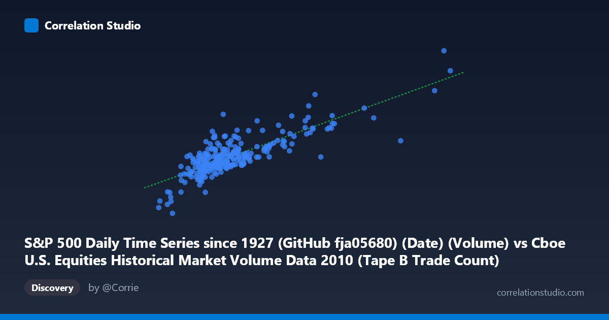
S&P 500 Daily Time Series since 1927 (GitHub fja05680) (Date) (Volume) vs Cboe U.S. Equities Historical Market Volume Data 2010 (Tape B Trade Count)
- Pearson correlation (r)
- 0.8152
- Spearman correlation
- 0.7304
- p-value
- 0
- Sample size (n)
- 252
- 95% confidence interval
- 0.7691 to 0.8529
- Granger causality
- None
- Granger optimal lag
- 10
AI analysis
Scatterplot Analysis: S&P 500 Daily Volume vs. Cboe Tape B Trade Count (2010)
Relationship Overview The scatterplot reveals a moderately strong positive relationship between S&P 500 daily trading volume and Cboe U.S. Equities Tape B trade count across the 2010 trading year. As daily market volume increases, the number of Tape B trades rises correspondingly, following a broadly linear trend captured by the regression equation y = 7,368.48x + 2.333B. This is an intuitively sensible pairing — both variables measure different dimensions of equity market activity on the same days, so co-movement reflects shared underlying market conditions (volatility spikes, macro events, institutional activity) rather than any surprising discovery.
Correlation Strength and Statistical Framing The Pearson correlation of r = 0.815 indicates a strong positive association, and the R² of 0.664 means that approximately 66.5% of the day-to-day variance in Tape B trade count is explained by overall market volume. While substantial, this also means roughly one-third of variation remains unexplained — likely attributable to exchange-specific routing decisions, fragmentation dynamics, or Tape B-listed security composition effects. The 95% confidence interval of [0.769, 0.853] is relatively tight given the sample of 252 trading days, and the p-value of effectively zero makes the correlation highly statistically significant, leaving no credible doubt about the existence of a positive relationship in the population. However, the Granger causality results tell a notably different story temporally: neither direction (X→Y: F=1.29, p=0.24; Y→X: F=0.48, p=0.90) achieves significance at the optimal 10-period lag. This means that while the two variables move together contemporaneously, past values of one do not meaningfully predict future values of the other — the relationship is synchronous co-movement, not temporal predictability.
Notable Patterns, Clusters, and Outliers The data display a fairly clean linear trend in the central mass, with the bulk of observations clustered between roughly 150,000–450,000 in volume and 3.0B–5.5B in trade count. However, several notable features stand out. A high-volume cluster in the upper-right (volumes ~500,000–920,000) shows elevated trade counts but with greater vertical scatter, suggesting the linear relationship becomes less precise at extreme volume levels. One conspicuous outlier sits near (918,660; 9.47B) — a day of exceptional volume accompanied by an outsized trade count that may correspond to a specific market stress event in 2010 (plausibly the May 6 Flash Crash or a heavy options expiration day). Conversely, a point near (134,700; 1.29B) represents the lowest activity day in the sample and sits close to the regression line, suggesting the linear model holds reasonably well at low-activity extremes. A modest fan-shaped spread (heteroscedasticity) appears to widen at higher volumes, which has implications for modeling precision.
Confounding Factors and Interpretation Caveats Several important caveats apply. First, both variables are simultaneously driven by the same market-wide conditions — volatility, macroeconomic news, Federal Reserve announcements, earnings seasons — making this partly a spurious correlation through a common driver rather than a direct causal link. Second, Tape B specifically covers NYSE American (AMEX) and regional exchange listings, so its trade count is also influenced by the composition and activity of Tape B-listed securities independent of broader S&P 500 volume. Third, the lack of Granger causality is a meaningful caution against any operational interpretation that one series leads the other; practitioners should not use lagged volume to forecast Tape B activity or vice versa with this data alone. Fourth, 2010 was a structurally unusual year — post-crisis market structure changes, high-frequency trading expansion, and the Flash Crash all distorted normal volume-trade count relationships. Results may not generalize to other periods.
Actionable Insights and Further Investigation For practitioners, the strong contemporaneous correlation suggests Tape B trade count could serve as a reasonable real-time proxy for broad market activity on an intraday or daily basis when direct volume figures are unavailable, though the ~33% unexplained variance warrants caution in precision-sensitive applications. Given the heteroscedasticity at high volumes, a log-log regression should be tested to assess whether a power-law relationship better captures the full range of the data. Analysts should isolate and investigate the extreme outlier to confirm whether it corresponds to the Flash Crash (May 6, 2010); if so, robust regression or outlier-adjusted models would provide cleaner baseline estimates. Extending the analysis to multiple years would test whether this relationship is stable across different market regimes or was idiosyncratic to 2010's specific structure. Finally, incorporating VIX or realized volatility as a third variable could help decompose how much of the co-movement is attributable to shared volatility sensitivity versus a more direct volume-to-trade-count mechanism.
X dataset: Cboe U.S. Equities Historical Market Volume Data 2010
Y dataset: S&P 500 Daily Time Series since 1927 (GitHub fja05680) (Date)
Part of experiment: Daily - Cboe U.S. Equities Historical Market Volume Data 2010 vs S&P 500 Daily Time Series since 1927 (GitHub fja05680) (Date)