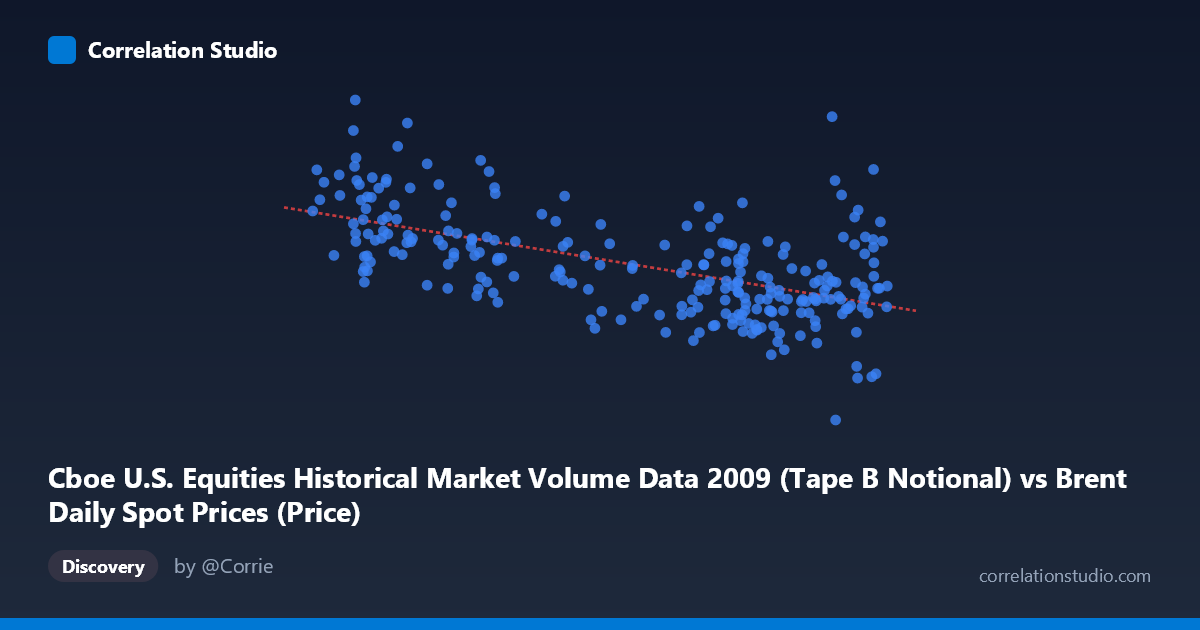
Cboe U.S. Equities Historical Market Volume Data 2009 (Tape B Notional) vs Brent Daily Spot Prices (Price)
- Pearson correlation (r)
- -0.5775
- Spearman correlation
- -0.5392
- p-value
- 0
- Sample size (n)
- 252
- 95% confidence interval
- -0.6544 to -0.4888
- Granger causality
- X → Y
- Granger optimal lag
- 10
AI analysis
Scatterplot Analysis: Brent Crude Oil Prices vs. Cboe Tape B Notional Volume (2009)
Relationship Overview The scatterplot reveals a moderate negative relationship between Brent crude oil spot prices (X-axis, in USD/barrel) and Cboe Tape B notional trading volume (Y-axis, in USD). The linear regression equation y = -6.126×10⁷x + 9.056×10⁹ indicates that for every $1/barrel increase in Brent crude prices, Tape B notional volume decreases by approximately $61.3 million. This inverse relationship is visually apparent across the 2009 trading year, spanning oil prices from roughly $39 to $79/barrel — a period that captured crude oil's dramatic recovery from its post-financial-crisis lows. The scatter is notably wide, however, suggesting the relationship, while real, is far from deterministic.
Correlation Strength and Statistical Significance The correlation coefficient of r = -0.5775 reflects a moderate negative association, but the more revealing metric is r² = 0.3335, meaning that oil price levels explain only about 33.3% of the variance in Tape B notional volume. The remaining ~67% is driven by factors entirely outside this model. The 95% confidence interval of [-0.6544, -0.4888] is meaningfully narrow given n = 252, and the p-value of effectively zero confirms this relationship is statistically robust and not a sampling artifact. Importantly, Granger causality runs unidirectionally from X→Y (F = 2.1672, p = 0.021) with an optimal lag of 10 trading periods (~2 weeks), meaning Brent crude price levels have statistically significant temporal predictive power over subsequent Tape B notional volume — while the reverse (Y→X: F = 1.309, p = 0.227) does not hold. This asymmetry is practically meaningful, though the modest F-statistic warrants cautious interpretation.
Notable Patterns, Clusters, and Outliers Several features stand out in the data sample. There is a visible cluster of high-volume observations ($7B notional) concentrated at lower oil price levels (~$42–$50/barrel), consistent with the early 2009 environment of peak financial-crisis volatility driving elevated equity trading activity. Conversely, as crude recovered toward $70–$78/barrel in the latter half of 2009, notional volumes generally compressed, though with substantial dispersion — for instance, points near x ≈ 77 show Y values ranging from roughly $2.4B to $7.7B, a spread of over $5B at the same price level. The observation at approximately (75.15, 1.32×10⁹) appears as a notable low-volume outlier and likely warrants investigation. This wide vertical spread at higher X values hints at heteroscedasticity, with variance in Y shrinking unevenly across the X range.
Confounding Factors and Interpretive Caveats This correlation almost certainly reflects shared dependence on a common underlying driver — the 2009 macroeconomic recovery narrative — rather than a direct causal mechanism between crude prices and Tape B equity volumes. Both series were heavily influenced by the post-Lehman recovery arc: early 2009 saw depressed oil prices alongside panic-driven high-frequency equity trading, while late 2009 saw stabilizing markets with normalized volumes. Tape B specifically covers regional exchange volume (not total U.S. equity volume), which may have its own structural dynamics related to market share shifts among exchanges in 2009. Additionally, the 10-period Granger lag, while statistically significant, could be capturing this shared macro momentum rather than a genuine informational transmission from energy markets to equity trading desks. Seasonal and day-of-week effects in both series also remain uncontrolled.
Actionable Insights and Further Investigation The Granger causality finding — that crude oil prices lead Tape B volume by ~10 trading days — is worth pursuing with a more robust vector autoregression (VAR) model controlling for broader market volatility (e.g., VIX), total U.S. equity market volume, and macro releases. Analysts should test whether this relationship persists across other years or is specific to the extreme 2009 regime; if it collapses outside crisis periods, the finding is contextually limited rather than structurally reliable. It would also be valuable to decompose Tape B volume into sectors to assess whether energy-sector equities are disproportionately driving the correlation. Finally, given the apparent heteroscedasticity and potential non-linearity visible at extreme X values, a log-transformed or piecewise regression may better characterize the relationship than the current linear specification.
X dataset: Brent Daily Spot Prices
Y dataset: Cboe U.S. Equities Historical Market Volume Data 2009
Part of experiment: Daily - Brent Daily Spot Prices vs Cboe U.S. Equities Historical Market Volume Data 2009