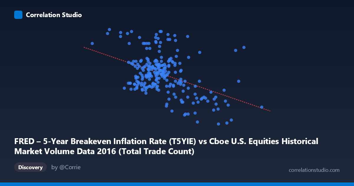
FRED – 5-Year Breakeven Inflation Rate (T5YIE) vs Cboe U.S. Equities Historical Market Volume Data 2016 (Total Trade Count)
- Pearson correlation (r)
- -0.4421
- Spearman correlation
- -0.3019
- p-value
- 0
- Sample size (n)
- 250
- 95% confidence interval
- -0.5367 to -0.3365
- Granger causality
- Y → X
- Granger optimal lag
- 1
AI analysis
Analysis: 5-Year Breakeven Inflation Rate vs. U.S. Equities Total Trade Count (2016)
Relationship Overview
The scatterplot reveals a moderate negative relationship between U.S. equity market trade counts (X-axis) and the 5-year breakeven inflation rate (Y-axis) across 2016. The linear regression equation (y = -1.63357E-07x + 1.82734) confirms that as daily trade counts increase, inflation expectations as measured by the breakeven rate tend to decline. Visually, the data points form a broadly downward-sloping cloud, though with considerable scatter around the trend line. The bulk of observations cluster in the 1.8M–3.2M trade count range with breakeven rates between roughly 1.25 and 1.70, suggesting a relatively stable central regime punctuated by notable deviations at the extremes.
Correlation Strength and Statistical Significance
The correlation coefficient of r = -0.4421 indicates a moderate negative association — meaningful but far from deterministic. Critically, r² = 0.1954 means that only ~19.5% of the variance in the breakeven inflation rate is explained by trade count volume, leaving roughly 80% of variation attributable to other factors. The 95% confidence interval of [-0.5367, -0.3365] is entirely negative and does not cross zero, reinforcing directional confidence, and the p-value of 2.194E-13 confirms this relationship is highly unlikely to be due to chance given the sample of 250 paired observations drawn from a population of 3,622. However, statistical significance here is partly a function of sample size and should not be conflated with practical or economic significance. The Granger causality results are particularly informative: Y (breakeven inflation rate) Granger-causes X (trade count) at a 1-period lag (F = 5.41, p = 0.021), while the reverse direction fails to reach significance (F = 1.42, p = 0.234). This unidirectional result suggests that inflation expectations have temporal predictive value for subsequent trading activity, not the other way around — a meaningful asymmetry for market participants.
Patterns, Clusters, and Outliers
Several features warrant attention. The central cluster (X ≈ 1.9M–2.5M, Y ≈ 1.40–1.60) is densely populated and relatively well-behaved, consistent with the typical trading environment during mid-2016. However, there are clear outliers: one observation near X ≈ 2.89M shows an unusually low breakeven rate of ~1.02, pulling strongly on the regression; another near X ≈ 2.37M registers a near-record-high breakeven of ~1.86. At the high end of trade counts, the point at X ≈ 4.14M with Y ≈ 1.70 and another at X ≈ 3.96M with Y ≈ 1.67 suggest that extreme volume days do not uniformly coincide with depressed inflation expectations, potentially indicating event-driven volume spikes. The low-volume, low-breakeven region (X < 1.7M, Y < 1.35) also forms a recognizable sub-cluster, possibly representing the early-2016 period when both market activity and inflation expectations were broadly suppressed.
Confounding Factors and Caveats
Several important caveats apply. First, the axes appear to be swapped in labeling relative to conventional analysis — trade count is listed as the X variable from the inflation dataset and vice versa, which may reflect a data pipeline labeling issue and warrants verification before drawing firm conclusions. Second, both variables are time-series in nature, meaning serial autocorrelation likely inflates the effective sample size and could overstate the precision of the confidence interval. Third, 2016 was an extraordinary year — it encompassed the Brexit vote (June), U.S. presidential election (November), and multiple Federal Reserve policy decisions — all of which independently influenced both equity trading volumes and inflation expectations, creating substantial omitted variable bias. The post-election "reflation trade" in late 2016 likely drove a simultaneous spike in both breakeven rates and volume, which could actually suppress or distort the underlying correlation. Finally, the Granger causality finding, while statistically suggestive, captures only linear temporal precedence at a 1-day lag and does not establish structural causation.
Actionable Insights and Further Investigation
The finding that inflation expectations Granger-cause trade activity at a 1-day lag is the most actionable result here. Market participants and quantitative analysts could explore whether daily changes in the T5YIE breakeven rate can serve as a short-horizon signal for equity market activity regime shifts — for instance, rapid moves in inflation expectations may precede elevated volume days worth positioning around. For further investigation, it would be valuable to: (1) decompose the analysis by sub-period (pre/post-Brexit, pre/post-election) to test whether the correlation is regime-dependent; (2) include additional controls such as VIX (volatility), Fed funds futures, or oil prices, which influence both breakeven rates and trading activity; (3) apply cointegration testing given both series are likely non-stationary; and (4) examine whether the relationship holds across different breakeven tenors (2-year, 10-year) to assess whether the 5-year horizon is uniquely predictive or part of a broader inflation-expectations-to-volume mechanism.
X dataset: Cboe U.S. Equities Historical Market Volume Data 2016
Y dataset: FRED – 5-Year Breakeven Inflation Rate
Part of experiment: Daily - Cboe U.S. Equities Historical Market Volume Data 2016 vs FRED – 5-Year Breakeven Inflation Rate