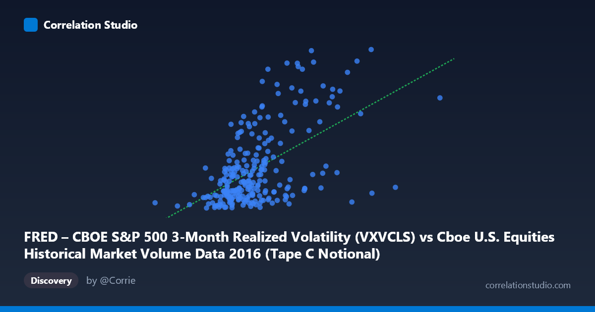
FRED – CBOE S&P 500 3-Month Realized Volatility (VXVCLS) vs Cboe U.S. Equities Historical Market Volume Data 2016 (Tape C Notional)
- Pearson correlation (r)
- 0.5467
- Spearman correlation
- 0.4902
- p-value
- 0
- Sample size (n)
- 252
- 95% confidence interval
- 0.4538 to 0.6279
- Granger causality
- None
- Granger optimal lag
- 1
AI analysis
Analysis: CBOE S&P 500 3-Month Realized Volatility vs. Tape C Notional Volume (2016)
Relationship Overview
The scatterplot reveals a moderate positive relationship between CBOE S&P 500 3-month realized volatility (VXVCLS) and Tape C notional trading volume across U.S. equity exchanges in 2016. As volatility rises, notional volume traded on Tape C venues tends to increase as well, consistent with the well-established finance intuition that heightened uncertainty drives greater trading activity. The linear regression equation (y = 1.457e-9·x + 10.999) confirms this positive slope, though the wide dispersion around the fitted line is immediately apparent, suggesting the relationship is real but far from deterministic.
Correlation Strength and Statistical Significance
The Pearson correlation of r = 0.547 indicates a moderate positive association, but the explained variance figure tells a more cautionary tale: R² = 0.299 means that roughly 30% of the variance in Tape C notional volume is attributable to VXVCLS, leaving approximately 70% unexplained by this single predictor. The 95% confidence interval for r [0.454, 0.628] is meaningfully bounded away from zero, and the p-value of effectively 0 (given n = 252 from a population of N = 3,622) confirms this is not a chance finding. However, the Granger causality results are notably weak in both directions — X→Y yields F = 0.007, p = 0.934, and Y→X yields F = 1.300, p = 0.255 — meaning that neither variable meaningfully predicts the other temporally at a 1-period lag. This is a critical finding: while the two variables move together contemporaneously, past volatility does not reliably forecast future volume, nor does past volume predict future volatility. The correlation reflects co-movement rather than a predictive or causal mechanism at daily frequency.
Notable Patterns, Clusters, and Outliers
Several structural features stand out in the data. The bulk of observations cluster at relatively lower volatility levels (roughly 3.5–5.5 billion on the X-axis) and lower Tape C notional values (15–20 range on Y), forming a dense core. However, there are clear high-leverage outliers in the upper-right quadrant — points near X = 7.3B with Y ≈ 24, and X = 6.2–6.4B with Y ≈ 26–27 — which likely correspond to specific market stress episodes in 2016 (e.g., Brexit in late June or the U.S. election in November). These outlier events appear to exert disproportionate influence on the regression slope and correlation coefficient. There is also some suggestion of heteroscedasticity: variance in Y appears to fan out at higher X values, which violates the homoscedasticity assumption of standard OLS regression and may inflate the apparent fit.
Confounding Factors and Caveats
Several important caveats apply. First, Tape C captures only a subset of total market notional volume (NYSE Arca-listed securities primarily), so the relationship may not generalize to the full U.S. equity market. Second, 2016 is a single calendar year containing discrete regime-shifting events (Brexit, the U.S. election), meaning the correlation may be heavily driven by a handful of episodic stress days rather than a stable structural relationship. Third, common drivers — such as macroeconomic announcements, Federal Reserve communications, or geopolitical shocks — likely cause both volatility and volume to spike simultaneously, making this a classic case of spurious co-movement due to shared external forcing rather than a direct link. Finally, the mismatch in dataset descriptions (axes appear to be labeled inversely relative to the column-to-axis mapping described) warrants verification before drawing firm conclusions.
Actionable Insights and Further Investigation
Practitioners should not use VXVCLS alone as a volume forecasting tool given the low R² and absent Granger causality. However, volatility regimes could serve as a useful conditioning variable: segmenting trading days into low-, medium-, and high-volatility regimes and modeling volume behavior within each regime may yield more actionable predictions. Further investigation should include: (1) extending the time series beyond 2016 to test whether the r ≈ 0.55 relationship is stable across different market regimes; (2) testing non-linear specifications (e.g., threshold or spline models) given the apparent heteroscedasticity; (3) incorporating VIX alongside VXVCLS to distinguish short- vs. medium-horizon volatility effects on volume; and (4) event-adjusting or windsorizing the Brexit and election outliers to assess their influence on the overall correlation. Understanding whether this relationship holds intraday or only at daily aggregation would also be valuable for market microstructure applications.
X dataset: Cboe U.S. Equities Historical Market Volume Data 2016
Y dataset: FRED – CBOE S&P 500 3-Month Realized Volatility
Part of experiment: Daily - Cboe U.S. Equities Historical Market Volume Data 2016 vs FRED – CBOE S&P 500 3-Month Realized Volatility