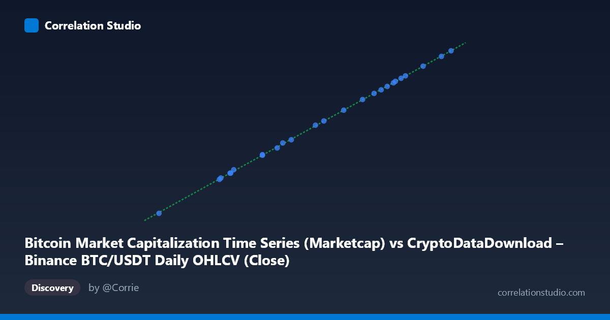
Bitcoin Market Capitalization Time Series (Marketcap) vs CryptoDataDownload – Binance BTC/USDT Daily OHLCV (Close)

Pearson correlation (r): 0.9999
Spearman correlation: 0.9985
p-value: 0
Sample size (n): 25
95% confidence interval: 0.9999 to 1
Granger causality: None
Granger optimal lag: 6

AI analysis

Analysis: Bitcoin Market Capitalization vs. BTC/USDT Close Price

1. Relationship Overview

This scatterplot is essentially a tautological relationship rather than an empirical correlation between two independent phenomena. Market capitalization is calculated as Price × Circulating Supply, so X (Marketcap) and Y (Close price) are mathematically derived from one another. With Bitcoin's circulating supply changing negligibly over this ~24-day window (only marginal new coin issuance), the two series move in near-perfect lockstep. The linear fit (y = 1.95183E+07x + 1.13243E+10) confirms this: the slope of ~19.5 million approximates the inverse of circulating supply at the time (~19.5 million BTC in circulation), which is exactly what we'd expect from the marketcap formula.

2. Strength, Direction, and Statistical Meaning

The correlation is essentially perfect: r = 0.9999, r² = 0.9999, meaning 99.99% of the variance in one variable is explained by the other. The 95% CI [0.9999, 1.0000] is vanishingly narrow, and the p-value of 0 indicates this relationship could not plausibly arise by chance. However, these statistics should be interpreted with the understanding that they reflect a definitional identity, not a causal or predictive economic relationship. This is reinforced by the Granger causality results: neither direction shows significant predictive power (X→Y: p=0.526; Y→X: p=0.529). This "non-finding" is expected — you cannot meaningfully "Granger-cause" a variable that is your own linear transformation with only a few days' lag; the contemporaneous identity dominates any lagged dynamics.

3. Patterns, Clusters, and Outliers

The data points trace a tight, linear band with no visible curvature, clusters, or outliers — consistent with a deterministic relationship rather than a noisy empirical one. Values span a relatively narrow range (X: ~61,277–71,620; a ~17% swing), reflecting a short, single-regime price trajectory over roughly one month (late March to late April 2024) without any regime shifts, crashes, or structural breaks visible in the sample. The absence of scatter around the regression line (R² ≈ 1) rules out any meaningful non-linear feature.

4. Confounding Factors and Caveats

The primary "caveat" here isn't a confound in the traditional sense — it's that the two variables are not independent measurements of related but distinct phenomena; they are two representations of the same underlying price series. Any apparent "relationship" is an artifact of data construction (marketcap = price × supply), not a discovery about market behavior. Treating this as evidence of a genuine economic relationship, running Granger causality tests, or computing confidence intervals as if these were independent time series is statistically valid mechanically but conceptually inappropriate — the near-zero Granger significance actually reflects the algorithm correctly detecting that there's no additional lagged information one series offers over the other, since they're contemporaneously identical up to a scale factor.

5. Actionable Recommendations

- Discard this pairing as an analytical exercise — comparing marketcap to price/close (from the same source) doesn't yield new insight; instead, pair marketcap against genuinely independent variables (trading volume, on-chain metrics, macro indicators like DXY or equity indices) to find meaningful relationships. - Verify circulating supply data: the near-fixed slope suggests supply was treated as constant; check if slight supply growth (~900 new BTC/day) should be modeled for precision in longer time horizons. - Extend the time window: a single month of tightly-trending data provides limited insight into volatility regimes; consider testing this identity across bull/bear cycles to confirm the relationship holds during high-volatility periods with supply shocks (e.g., post-halving effects). - Re-run Granger causality with truly independent series (e.g., price vs. exchange inflows, price vs. funding rates) where lead-lag dynamics would be economically meaningful.

X dataset: CryptoDataDownload – Binance BTC/USDT Daily OHLCV

Y dataset: Bitcoin Market Capitalization Time Series

Part of experiment: Bitcoin - CryptoDataDownload – Binance BTC/USDT Daily OHLCV vs Bitcoin Market Capitalization Time Series