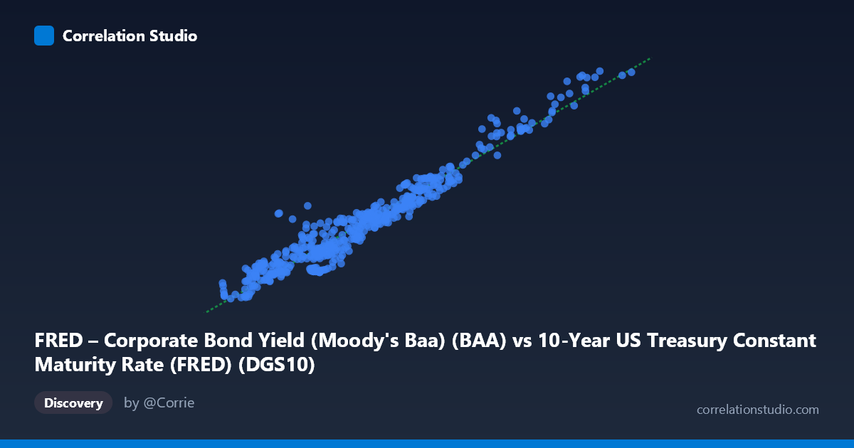
FRED – Corporate Bond Yield (Moody's Baa) (BAA) vs 10-Year US Treasury Constant Maturity Rate (FRED) (DGS10)
- Pearson correlation (r)
- 0.9672
- Spearman correlation
- 0.9464
- p-value
- 0
- Sample size (n)
- 492
- 95% confidence interval
- 0.9609 to 0.9724
- Granger causality
- None
- Granger optimal lag
- 1
AI analysis
Analysis: Moody's Baa Corporate Bond Yield vs. 10-Year US Treasury Yield
1. Overall Relationship
The scatterplot reveals a strikingly tight, positive linear relationship between the 10-Year US Treasury Constant Maturity Rate and Moody's Baa Corporate Bond Yield spanning over six decades (1962–2026). The data points cluster closely around the regression line (y = 0.952x + 2.304), indicating that as Treasury yields rise or fall, Baa corporate yields move in near-lockstep. This is economically intuitive: corporate bond yields are priced as a spread above the risk-free Treasury rate, so both instruments are driven by the same underlying interest rate environment. The intercept of approximately 2.30 percentage points effectively captures the long-run average credit spread embedded in Baa-rated (investment-grade but lower-tier) corporate debt.
2. Correlation Strength and Statistical Significance
The correlation is exceptionally strong at r = 0.9672, with r² = 0.9354, meaning approximately 93.5% of the variance in Baa corporate yields is explained by movements in the 10-Year Treasury yield alone. The 95% confidence interval for r is extremely narrow [0.9609, 0.9724], reflecting high precision from a large paired sample (n = 492, N = 1,288), and the p-value of effectively zero confirms this relationship is not a statistical artifact. The regression slope of 0.952 is close to—but slightly below—1.0, suggesting corporate yields rise somewhat less than one-for-one with Treasuries, likely because credit spreads compress slightly during rising-rate environments (which often coincide with economic expansions). However, the Granger causality tests reveal no significant temporal predictive direction in either direction (X→Y: F = 0.39, p = 0.53; Y→X: F = 0.35, p = 0.55), indicating that neither series reliably leads the other at a one-period lag. This is consistent with both yields being driven simultaneously by shared macro forces rather than one causing the other.
3. Patterns, Clusters, and Notable Features
The sample points span a wide dynamic range—from roughly (1.3, 3.2) at historic low-yield extremes to (14.05, 15.95) at the high-rate peaks characteristic of the early 1980s Volcker era—and the linear fit holds robustly across this entire range. There are no dramatic outliers that visually break from the trend, though some scatter is visible at lower yield levels (below x ≈ 3), where credit spread variability tends to be proportionally larger. The cluster of points in the x = 2–6 range reflects the prolonged post-2008 and post-2020 low-rate environments, while the upper-right cluster (x 10) corresponds to the inflationary 1970s–80s. The consistency of the relationship across such radically different monetary regimes is itself a notable finding, underscoring the structural nature of the Treasury-corporate yield linkage.
4. Confounding Factors and Caveats
Despite the high r², the remaining 6.5% unexplained variance is economically meaningful. Credit spreads—the gap between Baa and Treasury yields—are not constant; they widen significantly during recessions and financial crises (e.g., 2008–09, 2020) and compress during expansions. This means the relationship, while linear on average, contains cyclically driven heteroscedasticity that aggregated statistics may obscure. Additionally, the axes appear to be swapped in the dataset labeling (DGS10 is listed under the Baa dataset and vice versa), which warrants verification before drawing directional conclusions. Both series also share common data sources (FRED/Federal Reserve) and measurement conventions, potentially introducing correlated measurement characteristics. The Granger non-causality result should not be interpreted as independence—it simply means that at the tested lag, neither series provides incremental predictive power once its own history is accounted for.
5. Actionable Insights and Further Investigation
The near-unity slope and stable intercept (~230 basis points average spread) make this relationship a practical tool for credit spread monitoring: significant deviations of actual Baa yields from model-predicted values could signal changing credit risk conditions or anomalous monetary policy environments worth flagging. For further investigation, researchers should: (1) model the residuals (credit spreads) directly against macroeconomic variables such as unemployment, GDP growth, or VIX to explain the remaining variance; (2) conduct rolling-window correlation analysis to detect structural breaks or regime shifts (e.g., pre/post-2008); (3) test longer Granger lags (beyond 1 period) and higher-frequency data to more sensitively detect any lead-lag dynamics; and (4) extend the analysis to Aaa-rated bonds to decompose the Baa spread into a pure credit-risk component versus the broader rate environment, offering richer insight into investor risk appetite over time.
X dataset: 10-Year US Treasury Constant Maturity Rate (FRED)
Y dataset: FRED – Corporate Bond Yield (Moody's Baa)
Part of experiment: Daily - 10-Year US Treasury Constant Maturity Rate (FRED) vs FRED – Corporate Bond Yield (Moody's Baa)