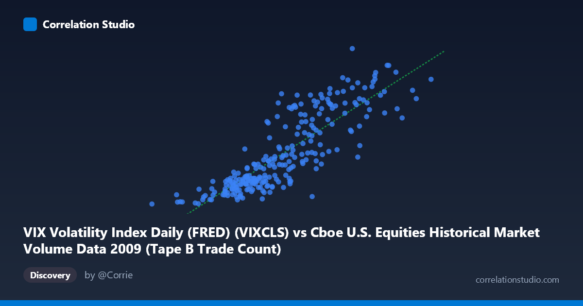
VIX Volatility Index Daily (FRED) (VIXCLS) vs Cboe U.S. Equities Historical Market Volume Data 2009 (Tape B Trade Count)
- Pearson correlation (r)
- 0.8494
- Spearman correlation
- 0.8665
- p-value
- 0
- Sample size (n)
- 252
- 95% confidence interval
- 0.811 to 0.8806
- Granger causality
- None
- Granger optimal lag
- 1
AI analysis
Analysis: VIX Volatility Index vs. Cboe Tape B Trade Count (2009)
Relationship Overview The scatterplot reveals a strong positive relationship between the VIX Volatility Index and Cboe Tape B trade count throughout 2009. As the VIX rises — indicating greater market fear and implied volatility — the number of Tape B trades increases substantially. This is intuitively coherent: periods of heightened market stress tend to drive elevated trading activity across equity exchanges, as market participants reposition, hedge, or react to rapidly changing conditions. The linear regression equation (y = 6.18×10⁻⁵x + 6.64) confirms that higher VIX values correspond to meaningfully higher trade counts, with the relationship appearing reasonably consistent across the observed range.
Correlation Strength and Statistical Interpretation The correlation is strong (r = 0.8494), and the r² of 0.7215 indicates that approximately 72% of the variance in Tape B trade count is statistically explained by the VIX level — a notably high proportion for financial market data. The 95% confidence interval [0.8110, 0.8806] is narrow relative to the estimate, reflecting high precision likely driven by the substantial sample size (n = 252 trading days, N = 3,232). The p-value of essentially zero confirms this is not a chance finding. However, the Granger causality results complicate the narrative considerably: neither X→Y (F = 0.0040, p = 0.9494) nor Y→X (F = 0.0287, p = 0.8656) shows any significant temporal predictive power at a 1-period lag. This means that while the two variables are strongly co-associated, neither reliably predicts the other on the following trading day — suggesting they move together contemporaneously, likely both driven by common underlying forces rather than one causing the other.
Notable Patterns, Clusters, and Outliers The sample points reveal a clear lower cluster — many observations concentrate below a VIX of ~30 and trade counts below ~350,000, corresponding to the relative market stabilization in the second half of 2009. A distinct upper cluster emerges above VIX 40, where trade counts escalate sharply toward 500,000–660,000+, likely reflecting the lingering volatility from the late 2008/early 2009 financial crisis. A few notable outliers are visible at the high end (e.g., ~766,764 trade count at VIX ~49; ~662,859 at VIX ~52), suggesting that at extreme fear levels, trading volume surges disproportionately. Interestingly, there is moderate vertical spread at mid-range VIX values (~25–35), indicating that the relationship is less deterministic in calmer periods, and other factors drive more of the variability there.
Confounding Factors and Caveats Several important caveats apply. First, 2009 is a structurally unusual year — it spans the tail of the Global Financial Crisis and the subsequent recovery, meaning the high-VIX/high-volume cluster may reflect a historically exceptional regime rather than a generalizable relationship. Second, both variables likely share common drivers (macro news shocks, Federal Reserve announcements, earnings seasons), which explains the high contemporaneous correlation without implying causation — consistent with the failed Granger tests. Third, Tape B specifically covers NYSE American (AMEX) and regional exchange trades, so its behavior may differ from Tape A or C; generalizing to total market volume requires caution. Finally, the optimal lag of only 1 period may be insufficient to capture slower-moving causal dynamics, and the absence of Granger causality at lag 1 does not rule out longer-horizon predictive relationships.
Actionable Insights and Further Investigation Practitioners monitoring market microstructure should note that VIX level is a strong contemporaneous signal for Tape B activity, useful for intraday capacity planning, liquidity provision strategies, and risk model calibration. However, since VIX does not Granger-cause trade counts at a 1-day lag, using yesterday's VIX to predict tomorrow's volume requires additional modeling. Recommended next steps include: (1) testing Granger causality at longer lags (5, 10, 22 days) to detect weekly or monthly predictive effects; (2) regime-splitting the data into crisis vs. recovery periods to assess whether the correlation holds outside extreme conditions; (3) comparing Tape A and Tape C trade counts against VIX to determine if this relationship is exchange-specific; and (4) incorporating additional covariates (S&P 500 returns, bid-ask spreads, Fed announcement calendars) to isolate the VIX-volume relationship from shared macro drivers and potentially recover the latent causal structure.
X dataset: Cboe U.S. Equities Historical Market Volume Data 2009
Y dataset: VIX Volatility Index Daily (FRED)
Part of experiment: Daily - Cboe U.S. Equities Historical Market Volume Data 2009 vs VIX Volatility Index Daily (FRED)