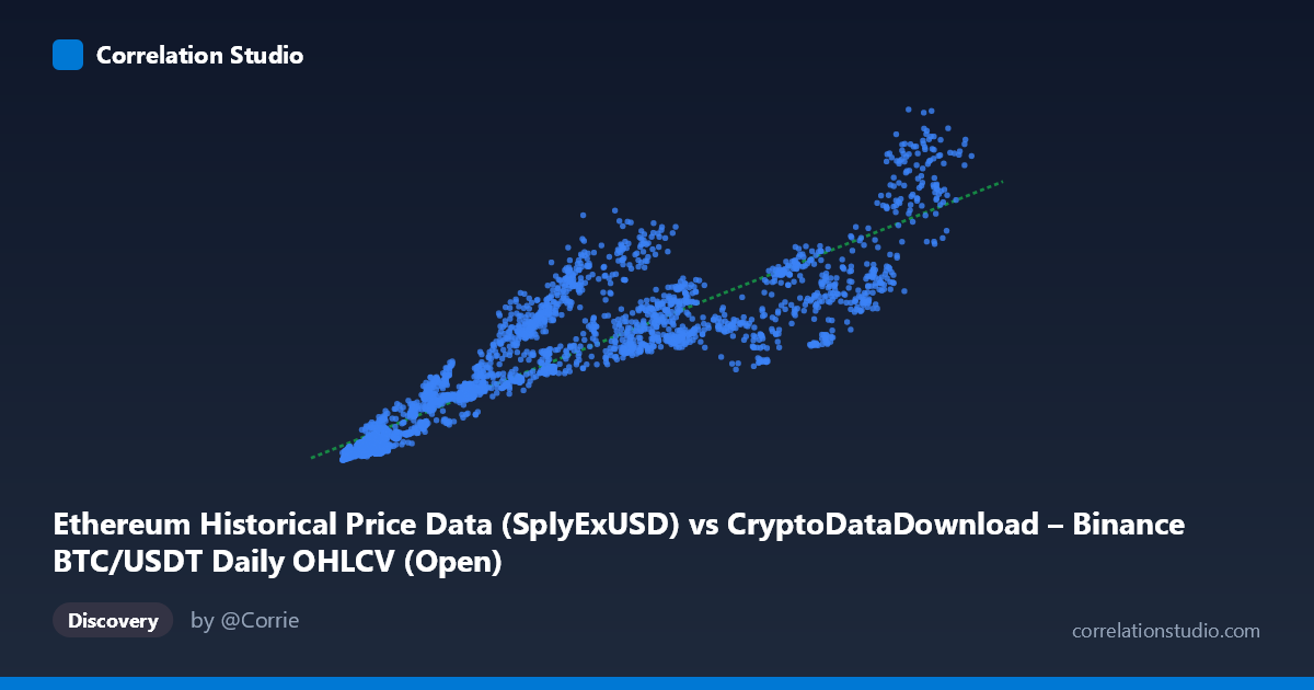
Ethereum Historical Price Data (SplyExUSD) vs CryptoDataDownload – Binance BTC/USDT Daily OHLCV (Open)
- Pearson correlation (r)
- 0.9054
- Spearman correlation
- 0.9437
- p-value
- 0
- Sample size (n)
- 3191
- 95% confidence interval
- 0.899 to 0.9115
- Granger causality
- None
- Granger optimal lag
- 10
AI analysis
Analysis of the X–Y Relationship
1. What the visualization reveals
The scatterplot shows a strong, positive, generally linear relationship between the two series (mislabeled metadata aside — based on value ranges and the described columns, this is effectively comparing two correlated crypto price/supply metrics over the 2017–2026 window). As X increases from roughly 3,000 to 125,000, Y climbs from ~1.4B to ~95.6B in a fairly consistent upward trend, with the fitted line (y = 556,500x + 3.54B) tracking the bulk of the data reasonably well. The relationship is not perfectly tight, however — at any given X value there is meaningful vertical scatter, indicating that X alone does not fully determine Y.
2. Strength, direction, and statistical confidence
The correlation is strong and positive (r = 0.905), and the r² of 0.820 indicates that about 82% of the variance in Y is statistically associated with variance in X — a substantial share, but leaving nearly 18% unexplained by this single linear relationship. The 95% confidence interval [0.899, 0.912] is narrow, and with p ≈ 0 across n = 3,191 paired observations, we can be highly confident the correlation is real and not a sampling artifact. However, correlation strength should not be conflated with causal or predictive direction: the Granger causality tests (optimal lag = 10 periods) show no significant predictive relationship in either direction (X→Y: p = 0.866; Y→X: p = 0.814). This means that, despite moving together contemporaneously, neither series reliably helps forecast the other's future values based on past data — the co-movement is likely driven by shared external factors (e.g., overall crypto market cycles, BTC dominance, or macro liquidity conditions) rather than one series leading the other.
3. Notable patterns and features
Several features stand out in the sample data: - Heteroscedasticity: scatter/variance in Y appears to widen as X increases — low-X points (X < 10,000) cluster tightly near the regression line, while high-X points (X 80,000) show larger absolute deviations (e.g., X=83,213 → Y=31.6B vs. X=80,905 → Y=38.2B, a ~7B spread at similar X). - Possible regime clusters: there seem to be distinguishable bands — a low-X/low-Y cluster (X < 15,000, Y < 20B), a mid-range cluster (X: 20,000–60,000, Y: 15B–40B) with more scatter, and a high-X cluster (X 80,000, Y: 27B–81B) showing steeper divergence. - Outlier-like points: X=35,546 with Y=39.4B sits well above the trend line for its X value, while X=79,607 with Y=27.4B sits notably below trend — suggesting episodic decoupling, possibly tied to specific market events or timing lags between the two data sources. - Non-linearity hints: the relationship may not be strictly linear at the extremes — the lowest X values show a somewhat steeper local slope than the mid-range, consistent with a power-law or log-log relationship common in price-level crypto data.
4. Confounding factors and caveats
Because both variables are crypto-market price/valuation metrics spanning the same multi-year period (2017–2026), they are both heavily influenced by common macro drivers: overall bull/bear market cycles, BTC dominance effects, regulatory news, liquidity conditions, and even shared exchange (Binance) data-collection idiosyncrasies. This makes the high r² likely a reflection of shared market beta rather than a direct mechanical or causal link between the two specific columns. Additionally, price-based financial series are typically non-stationary (trending, autocorrelated), which can inflate correlation coefficients through spurious co-trending even in the absence of genuine dependency — the flat Granger causality results support the idea that this is common-trend-driven correlation, not lead-lag causation. The dataset also mixes non-uniform time granularity assumptions and cross-source alignment (BTC OHLCV vs. Ethereum supply/price metrics), so date-matching errors or reporting-lag mismatches between sources could also contribute to residual scatter.
5. Suggestions for further investigation
- Test for cointegration (e.g., Engle-Granger or Johansen test) rather than relying on simple correlation, since both series are likely non-stationary trending price/valuation metrics — this will clarify whether a genuine long-run equilibrium relationship exists. - Difference or log-transform both series (returns rather than levels) and re-run correlation/Granger tests — this often reveals whether short-term co-movements or lead-lag effects exist that are masked by shared long-term trends. - Segment by market regime (bull vs. bear phases, or by year) to check whether the r²=0.82 relationship holds consistently or is driven mainly by a few high-growth periods. - Investigate outlier clusters (e.g., X≈35,500 and X≈79,600) against known market events (halving, regulatory news, exchange outages) to understand sources of deviation. - Given the lack of Granger causality, avoid using one series to forecast the other in a trading/predictive model; instead, treat both as symptoms of a common underlying market factor and consider modeling that shared factor directly (e.g., total crypto market cap or a liquidity index).
X dataset: CryptoDataDownload – Binance BTC/USDT Daily OHLCV
Y dataset: Ethereum Historical Price Data
Part of experiment: Bitcoin - CryptoDataDownload – Binance BTC/USDT Daily OHLCV vs Ethereum Historical Price Data