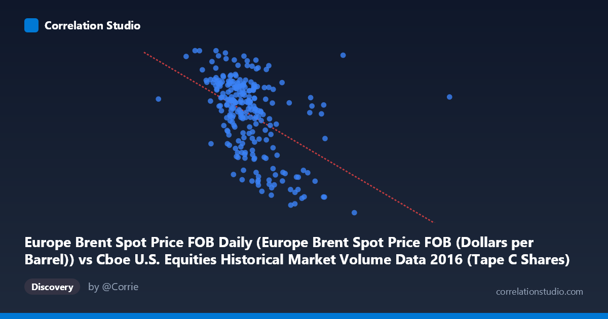
Europe Brent Spot Price FOB Daily (Europe Brent Spot Price FOB (Dollars per Barrel)) vs Cboe U.S. Equities Historical Market Volume Data 2016 (Tape C Shares)
- Pearson correlation (r)
- -0.4706
- Spearman correlation
- -0.4989
- p-value
- 0
- Sample size (n)
- 251
- 95% confidence interval
- -0.5617 to -0.3683
- Granger causality
- None
- Granger optimal lag
- 1
AI analysis
Analysis: Europe Brent Spot Price vs. Cboe Tape C Share Volume (2016)
Relationship Overview The scatterplot reveals a negative relationship between Europe Brent Spot Price (X-axis, in dollars per barrel) and Cboe Tape C share volume (Y-axis, in shares). As oil prices increase, Tape C equity trading volume tends to decrease, and vice versa. The linear regression equation (y = -1.158E-07x + 59.07) confirms this inverse slope, suggesting that for every ~$8.65 increase in oil price, Tape C volume declines by approximately one unit. The relationship is visually apparent but noisy, with considerable scatter around the regression line, indicating that oil price alone is far from a complete explanation of trading volume behavior.
Correlation Strength and Statistical Significance The Pearson correlation of r = -0.4706 reflects a moderate negative association. However, the explanatory power is limited: R² = 0.2215, meaning oil prices account for only about 22% of the variance in Tape C volume, leaving roughly 78% explained by other factors. The 95% confidence interval of [-0.5617, -0.3683] is entirely negative and does not cross zero, reinforcing directional confidence. The p-value of 3.1E-15 is extraordinarily small given n = 251, confirming this is almost certainly not a chance correlation. Critically, however, Granger causality testing finds no significant predictive direction in either direction (X→Y: F = 1.41, p = 0.24; Y→X: F = 0.016, p = 0.90). This means that despite a meaningful contemporaneous correlation, neither variable reliably predicts the other temporally — the relationship does not carry actionable lead-lag forecasting power at a one-period lag.
Notable Patterns, Clusters, and Outliers Several structural features are visible in the data. The bulk of observations cluster in the X range of roughly 100M–150M, corresponding to mid-range oil prices (~40–52 $/barrel), forming a dense core with moderate vertical spread. There are notable low-volume outliers at higher oil price values: points near X = 175M and X = 229M (oil prices around $27–28/barrel) show very low Tape C volume (~26–28), dragging the regression line strongly. These extreme low-price, low-volume points — likely corresponding to the early 2016 oil price trough — may be exerting disproportionate leverage on the correlation. Additionally, several high-volume points (Y 52) appear at lower X values, suggesting volume spikes may cluster around periods of market stress or oil price uncertainty.
Confounding Factors and Caveats This correlation likely reflects shared exposure to broader macroeconomic conditions rather than a direct causal mechanism between oil prices and Tape C volume. Early 2016 was characterized by simultaneous equity market turbulence, risk-off sentiment, and an oil price crash — conditions that could independently suppress both variables or create spurious co-movement. Tape C volume specifically covers NYSE Arca-listed securities (including many ETFs and energy-related instruments), which may have an elevated structural sensitivity to oil market conditions compared to other tapes. Furthermore, the dataset spans only one calendar year (2016), limiting generalizability; the correlation structure observed here may not persist across different market regimes. The mismatch between column descriptions (X and Y labels appear swapped in the dataset notes) also warrants verification before drawing firm conclusions.
Actionable Insights and Further Investigation Given that the correlation is statistically robust but causally ambiguous and temporally non-predictive, practitioners should treat oil price as a contemporaneous risk indicator for Tape C volume rather than a forecasting signal. Several follow-up analyses are recommended: (1) Extend the time series beyond 2016 to test whether the negative correlation is regime-specific or structural; (2) Segment by market regime (e.g., high-VIX vs. low-VIX periods) to test whether volatility is a hidden common driver; (3) Test longer Granger lags (2–5 periods) since the optimal lag of 1 may be insufficient; (4) Examine other tape volumes (Tape A, B) to determine whether this relationship is unique to Tape C's instrument composition; and (5) consider multivariate regression incorporating VIX, S&P 500 returns, and USD index to properly isolate the oil price effect on trading volume.
X dataset: Cboe U.S. Equities Historical Market Volume Data 2016
Y dataset: Europe Brent Spot Price FOB Daily
Part of experiment: Daily - Cboe U.S. Equities Historical Market Volume Data 2016 vs Europe Brent Spot Price FOB Daily