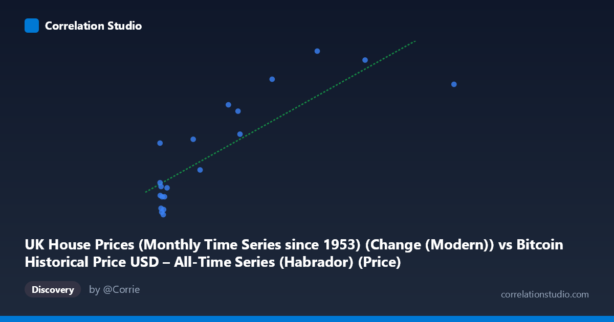
UK House Prices (Monthly Time Series since 1953) (Change (Modern)) vs Bitcoin Historical Price USD – All-Time Series (Habrador) (Price)
- Pearson correlation (r)
- 0.8368
- Spearman correlation
- 0.7142
- p-value
- 0.000004
- Sample size (n)
- 20
- 95% confidence interval
- 0.6261 to 0.9336
- Granger causality
- None
- Granger optimal lag
- 5
- Time coverage
- 2010-08-01 to 2015-05-01
- Recomputed on refreshed data
- 2026-10-24 (r was 0.8368)
AI analysis
Analysis: Bitcoin Price vs. UK House Price Change (Modern Series)
1. What the Visualization Reveals
The scatterplot shows a clear positive, roughly linear relationship between the two variables: as the X-value (labeled here as Bitcoin price, though the axis metadata is cross-labeled with UK house prices — see caveats below) increases, the Y-value tends to rise as well. Points cluster densely at low X-values (under ~50) with Y-values ranging from about -1.8 to 4, while higher X-values (200–850) correspond consistently to higher Y-values (6.3–11.0). This creates a visible upward-sloping band consistent with the fitted regression line (y = 0.0151x + 0.597).
2. Strength, Direction, and Statistical Confidence
The correlation coefficient (r = 0.837) indicates a strong positive linear relationship, and r² = 0.700 means 70% of the variance in Y is statistically explained by X — a substantial share, though 30% remains unexplained by this simple linear model. The 95% CI for r [0.626, 0.934] is fairly wide (reflecting the small sample, n=20) but excludes zero entirely, and the p-value (4.25×10⁻⁶) is highly significant, giving strong confidence that this correlation is not due to chance. However, the Granger causality tests tell a different story: neither direction (X→Y: p=0.247; Y→X: p=0.775) shows significant predictive causality at the optimal lag of 5 periods. This means that despite the strong contemporaneous correlation, there is no statistical evidence that movements in one series temporally precede or predict movements in the other — the relationship may be coincidental, driven by a shared underlying trend (e.g., both increasing over the 2010–2015 window), rather than a causal lead-lag dynamic.
3. Notable Patterns and Outliers
Most low-X points sit near Y=0, with a tight sub-cluster of small negative Y-values (-1.8 to -0.3) for X between 0.7 and 20 — suggesting a floor effect or a distinct low-value regime. A few points deviate from the linear trend: (96.42, 4.10) and (116.38, 1.70) sit below where the line would predict, while (0.06, 3.80) is a clear outlier — an extremely low X paired with a moderately high Y, breaking the otherwise consistent low-X/low-Y pattern. The very high end of X (853.02, 595.08, 456.27) does follow the trend reasonably well, supporting the linear fit at the extremes, though sparse sampling there limits confidence in that region's exact slope.
4. Confounding Factors and Caveats
The most critical caveat is the axis labeling itself: the metadata shows the X-axis and Y-axis dataset descriptions are swapped/cross-referenced (X is labeled "UK House Prices" but described as Bitcoin price data, and vice versa for Y), suggesting a data-pipeline labeling error that should be resolved before drawing conclusions. Additionally, both Bitcoin price and UK house prices were on general upward trajectories during 2010–2015 due to independent macroeconomic factors (Bitcoin adoption cycles vs. UK monetary policy/post-recession recovery) — a classic case of two non-stationary trending series producing "spurious correlation" without genuine mechanistic linkage. With only n=20 paired points sampled from a population of 290, and monthly time-series data likely exhibiting autocorrelation, the effective independent sample size is smaller than it appears, inflating apparent significance.
5. Recommendations for Further Investigation
First, verify and correct the axis/column labeling to ensure the correlation is being interpreted for the correct variable pairing. Second, test both series for stationarity (e.g., ADF test) and consider using differenced or detrended series rather than raw levels to rule out spurious trend-driven correlation. Third, given the null Granger causality result, avoid using one series to forecast the other in a trading or economic model — instead, treat the correlation as descriptive/co-trending rather than predictive. Finally, expanding the sample size beyond n=20 (the full population has 290 points) and testing sub-periods would help determine whether the relationship is stable over time or an artifact of the specific 2010–2015 bull-market window.
X dataset: Bitcoin Historical Price USD – All-Time Series (Habrador)
Y dataset: UK House Prices (Monthly Time Series since 1953)
Part of experiment: Bitcoin - Bitcoin Historical Price USD – All-Time Series (Habrador) vs UK House Prices (Monthly Time Series since 1953)