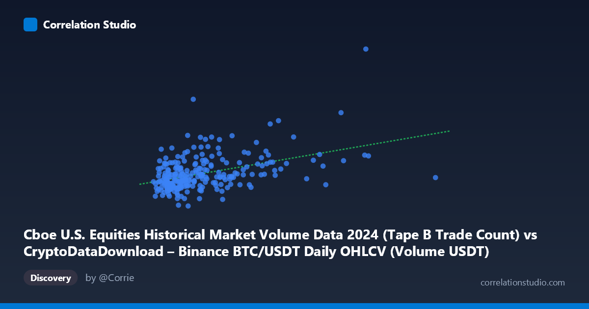
Cboe U.S. Equities Historical Market Volume Data 2024 (Tape B Trade Count) vs CryptoDataDownload – Binance BTC/USDT Daily OHLCV (Volume USDT)
- Pearson correlation (r)
- 0.4323
- Spearman correlation
- 0.3883
- p-value
- 0
- Sample size (n)
- 252
- 95% confidence interval
- 0.3261 to 0.5277
- Granger causality
- None
- Granger optimal lag
- 10
- Time coverage
- 2024-01-02 to 2024-12-31
AI analysis
Analysis: Cboe Trade Count vs. Binance BTC/USDT Volume (USDT)
1. Overview of the Relationship
The scatterplot shows a modest positive association between Cboe U.S. equities trade counts (X) and Binance BTC/USDT trading volume in USDT (Y). Most points cluster in the lower-left region of the plot (X between ~1.2B and ~4B, Y between ~280K and ~600K), indicating that on the majority of trading days, both variables occupy a relatively narrow, low-to-moderate range. A handful of points extend the X-axis considerably (up to ~11B), and one dramatic outlier reaches Y ≈ 1,170,416 at X ≈ 8.58B, pulling the regression line's slope upward.
2. Strength, Direction, and Uncertainty
The correlation coefficient (r = 0.432) indicates a weak-to-moderate positive linear relationship. Critically, r² = 0.187 means only 18.7% of the variance in Binance USDT volume is explained by Cboe trade counts — leaving over 80% of Y's variability attributable to other factors. The 95% CI for r [0.326, 0.528] is reasonably tight and excludes zero, and the p-value (6.7×10⁻¹³) confirms the correlation is highly statistically significant — this is a real, non-random pattern, not noise. However, statistical significance here reflects the large-ish sample size (n=252) detecting a genuine but practically weak effect, not a strong predictive relationship. The Granger causality tests reinforce this: neither direction (X→Y or Y→X) shows significant predictive power at the optimal 10-day lag (both p 0.84), meaning past values of one series do not meaningfully forecast future values of the other. This suggests the correlation is likely contemporaneous/coincidental (e.g., both markets reacting to shared macro conditions) rather than one market leading the other.
3. Patterns, Clusters, and Outliers
The data shows a dense, roughly linear-looking core cluster below X = 4B, with substantial scatter in Y (300K–700K) that isn't tightly tracking X. Beyond X = 4B, points become sparse — a handful of days with unusually high Cboe trade counts (5.5B, 6.7B, 8.6B, 11B) act as high-leverage points. The extreme outlier at (8.58B, 1,170,416) stands out sharply from the rest of the distribution and likely exerts disproportionate influence on both the slope and r² — this could correspond to a specific high-volatility event (e.g., a major BTC price move or equities volume spike, possibly around elections, Fed announcements, or crypto-specific news in 2024). Without this point, the already-modest correlation might weaken further.
4. Confounding Factors and Caveats
Several caveats limit causal interpretation: - Spurious correlation risk: Both series may be driven by common macro drivers (overall market volatility, risk sentiment, major news days) rather than a direct mechanical link between equities trade counts and crypto volume. - Leverage/outlier sensitivity: With only 252 points and at least one extreme outlier, r² and the regression slope are vulnerable to distortion — a robustness check (e.g., Spearman correlation, outlier-trimmed regression) is warranted. - Non-stationarity: Both volume series likely exhibit trends, volatility clustering, and autocorrelation typical of financial time series, which can inflate apparent correlation in ways that don't reflect true dependency (the Granger test result actually supports this concern). - Mismatched economic meaning: Trade count (X) and dollar volume (Y) are different units of market activity intensity; scaling effects (e.g., average trade size differences between equities and crypto markets) may not be directly comparable.
5. Recommendations for Further Investigation
- Test with outliers removed to see how much the extreme point(s) drive r and the regression slope. - Use log-transformed variables given the strong right-skew in both X and Y (as evidenced by the wide range vs. mean/stdev) — this often clarifies whether the relationship is genuinely linear or exponential/multiplicative. - Investigate specific dates of high-X, high-Y points to identify shared macro events (e.g., FOMC days, ETF approval news, quad-witching days) that might explain co-movement without direct causality. - Given the null Granger result, this pair should not be used for lead-lag trading signals; instead, treat any comovement as coincidental/contemporaneous, and explore a shared third-factor model (e.g., VIX, overall market volatility index) as a more promising causal driver.
X dataset: CryptoDataDownload – Binance BTC/USDT Daily OHLCV
Y dataset: Cboe U.S. Equities Historical Market Volume Data 2024
Part of experiment: Bitcoin - CryptoDataDownload – Binance BTC/USDT Daily OHLCV vs Cboe U.S. Equities Historical Market Volume Data 2024