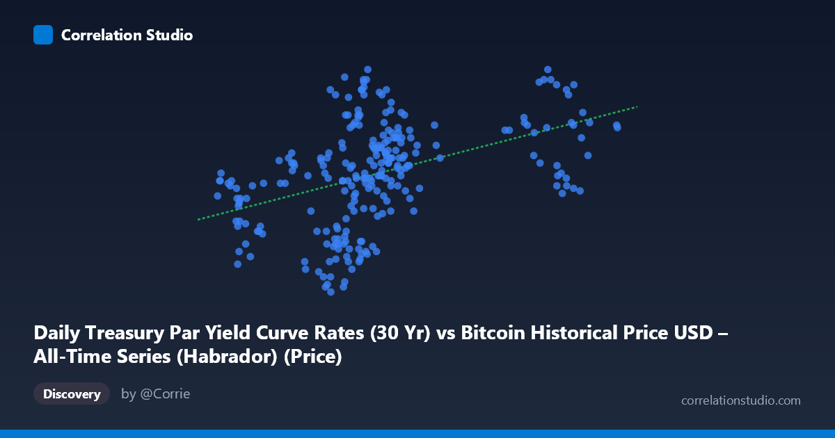
Daily Treasury Par Yield Curve Rates (30 Yr) vs Bitcoin Historical Price USD – All-Time Series (Habrador) (Price)
- Pearson correlation (r)
- 0.4347
- Spearman correlation
- 0.5022
- p-value
- 0
- Sample size (n)
- 250
- 95% confidence interval
- 0.3283 to 0.5301
- Granger causality
- None
- Granger optimal lag
- 1
AI analysis
Analysis: Treasury 30-Yr Yield vs. Bitcoin Price Relationship
1. Overview of the Relationship
The scatterplot shows a moderate positive relationship between the 30-Year Treasury yield (X-axis) and Bitcoin price (Y-axis) across 250 daily observations from 2024. As Treasury yields rise from roughly 39,500 to 106,000 (basis points or scaled units), Bitcoin prices tend to drift upward from the mid-3.9 range to nearly 4.8. The regression line (y = 6.108E-06x + 4.0049) confirms this upward trend, but the scatter around the line is substantial, indicating the relationship is far from deterministic.
2. Strength, Direction, and Statistical Confidence
The correlation coefficient (r = 0.4347) indicates a moderate positive linear relationship, but r² = 0.1889 reveals that only 18.9% of the variance in Bitcoin price is explained by movements in the Treasury yield — meaning over 80% of Bitcoin's price variation stems from other factors entirely. The 95% confidence interval [0.328, 0.530] is reasonably tight and does not cross zero, and the p-value (6.06E-13) is highly significant, confirming this correlation is not due to chance in this sample. However, statistical significance with a large N (250) is expected even for modest effect sizes — significance does not imply practical strength. Critically, the Granger causality tests show no significant predictive direction in either direction (X→Y: p=0.409; Y→X: p=0.128), meaning neither series reliably helps forecast the other's future values based on past data. This suggests the correlation is likely driven by both variables trending together over 2024 (e.g., a common macro backdrop) rather than one causing or forecasting the other.
3. Patterns and Clusters in the Data
The data shows a dense cluster in the lower X-range (roughly 55,000–70,000) with Y-values spanning widely from 3.94 to 4.78, indicating high variance at similar X levels. A second, sparser cluster exists at higher X-values (85,000–106,000), where Y-values are consistently in the 4.4–4.8 range with less spread. This pattern hints at a non-linear or regime-shift structure: at lower X, Y is highly variable and includes the dataset's lowest values (3.94–4.14), while at higher X, Y stabilizes at elevated levels. This could suggest a threshold effect rather than a purely linear relationship, or simply reflects fewer observations at high X reducing apparent variance.
4. Confounding Factors and Caveats
Several caveats apply. First, both series are time-ordered financial/economic data from the same year, and both may be correlated with a common macro driver (e.g., Fed policy, inflation expectations, risk sentiment) rather than one directly influencing the other — the null Granger causality result supports this "spurious co-trending" interpretation. Second, financial time series often exhibit autocorrelation (today's value close to yesterday's), which inflates apparent correlation between any two trending series without implying a genuine relationship — this is a classic time-series pitfall. Third, the uneven sampling density (dense at low X, sparse at high X) could distort the correlation estimate and give undue leverage to a handful of high-X points (e.g., the ~92,982–101,100 cluster).
5. Actionable Insights and Next Steps
Given the weak explanatory power (r²=0.19) and lack of Granger causality, this correlation should not be used for predictive trading or forecasting models linking Treasury yields to Bitcoin price. Instead, analysts should: (a) test for a common confounding macro variable (e.g., DXY, Fed funds rate, or inflation data) using multivariate regression; (b) apply differencing or detrending to both series to check if the correlation persists after removing shared trend components (a standard remedy for spurious time-series correlation); (c) investigate the apparent regime shift near X≈85,000 with segmented/piecewise regression to see if a non-linear model fits better; and (d) extend the analysis with additional lags or a Vector Autoregression (VAR) framework to more rigorously rule out delayed causal effects beyond the single-lag test performed here.
X dataset: Bitcoin Historical Price USD – All-Time Series (Habrador)
Y dataset: Daily Treasury Par Yield Curve Rates
Part of experiment: Bitcoin - Bitcoin Historical Price USD – All-Time Series (Habrador) vs Daily Treasury Par Yield Curve Rates