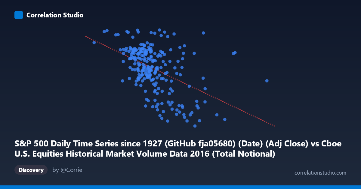
S&P 500 Daily Time Series since 1927 (GitHub fja05680) (Date) (Adj Close) vs Cboe U.S. Equities Historical Market Volume Data 2016 (Total Notional)

Pearson correlation (r): -0.4757
Spearman correlation: -0.4655
p-value: 0
Sample size (n): 252
95% confidence interval: -0.566 to -0.3742
Granger causality: None
Granger optimal lag: 4

AI analysis

Analysis: S&P 500 Adjusted Close vs. Total Market Notional Volume (2016)

Relationship Overview The scatterplot reveals a moderate negative relationship between the S&P 500 adjusted closing price and total U.S. equities market notional volume throughout 2016. As the S&P 500 index level rises, total notional trading volume tends to decline, and conversely, periods of lower index prices coincide with elevated trading volumes. This is an economically intuitive finding: market stress, corrections, and volatility episodes typically drive heightened trading activity, while calmer, steadily rising markets are often accompanied by reduced turnover. The linear regression equation (y = -1.134×10⁻⁸x + 2310.16) confirms this inverse slope, though the relationship is far from deterministic.

Correlation Strength and Statistical Significance The Pearson correlation of r = -0.4757 indicates a moderate negative association. Crucially, the R² of 0.2263 means that S&P 500 price level explains only about 22.6% of the variance in total notional volume — leaving roughly 77% of volume variation unexplained by price alone. The 95% confidence interval of [-0.566, -0.374] is meaningfully negative throughout, and the p-value of 1.33×10⁻¹⁵ confirms this is extremely unlikely to be a chance finding at any conventional significance threshold. However, statistical significance here is partly a function of the large population size (N = 3,622). Despite the robust correlation signal, the Granger causality tests tell a different story: neither direction (X→Y nor Y→X) achieves significance (F = 0.46, p = 0.77 and F = 0.99, p = 0.41, respectively, at optimal lag 4). This means that past S&P 500 prices do not reliably predict future notional volume, and vice versa — the relationship is contemporaneous and associative rather than temporally predictive.

Notable Patterns, Clusters, and Outliers Several features stand out in the sample points. There is a visible cluster of high-volume, lower-price observations — points with X values in the 23–26 billion range tend to show Y (S&P prices) in the 1,868–1,940 range, consistent with early 2016 market turbulence and the February correction. Conversely, a dense cluster of moderate-to-high price points (S&P ~2,050–2,200) congregates in the 14–20 billion notional volume range, reflecting the calmer mid-to-late 2016 environment. Potential outliers include the point near (13,956,072,697, 2,265.18) — unusually low volume paired with a near-peak price — and (21,239,466,584, 2,262.03), which shows high volume at high price, possibly reflecting the post-election rally surge in November 2016 where both price and activity spiked simultaneously. These outliers hint at non-linearity: the inverse relationship weakens or reverses at extreme price highs driven by exogenous shocks.

Confounding Factors and Caveats Several confounds complicate causal interpretation. Volatility (VIX) is a well-known volume driver independent of price level, and both variables here likely share volatility as a common cause. The time dimension is critical: 2016 contains distinct regimes (early-year selloff, mid-year Brexit shock, late-year U.S. election rally), and pooling these creates a spurious structure. Seasonal and calendar effects — month-end rebalancing, quarterly options expiration, holiday-shortened weeks — can independently inflate or deflate both variables. Additionally, the notional volume metric is sensitive to price level by construction (shares traded × price), introducing a mechanical circularity: higher index prices inflate notional values even at constant share volumes, which could partially suppress the negative coefficient rather than amplify it. The dataset's single-year scope also limits generalizability.

Actionable Insights and Further Investigation Practitioners should not use S&P 500 price level as a standalone predictor of notional volume given the weak Granger causality and modest R². More productive avenues include: (1) controlling for realized volatility or VIX to isolate the price-volume relationship from the volatility channel; (2) decomposing notional volume into share volume × average price to disentangle mechanical from behavioral effects; (3) segmenting by market regime (e.g., trending vs. mean-reverting, pre/post-election) to test whether the correlation is regime-dependent; (4) extending the time series across multiple years to test whether 2016's pattern is idiosyncratic to that year's specific macro events; and (5) exploring nonlinear models (e.g., piecewise regression or LOESS smoothing) to capture the evident heteroscedasticity and cluster structure visible in the chart.

X dataset: Cboe U.S. Equities Historical Market Volume Data 2016

Y dataset: S&P 500 Daily Time Series since 1927 (GitHub fja05680) (Date)

Part of experiment: Daily - Cboe U.S. Equities Historical Market Volume Data 2016 vs S&P 500 Daily Time Series since 1927 (GitHub fja05680) (Date)