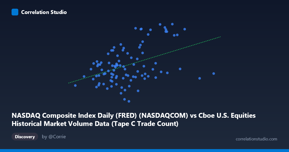
NASDAQ Composite Index Daily (FRED) (NASDAQCOM) vs Cboe U.S. Equities Historical Market Volume Data (Tape C Trade Count)
- Pearson correlation (r)
- 0.4251
- Spearman correlation
- 0.3471
- p-value
- 0.000012
- Sample size (n)
- 99
- 95% confidence interval
- 0.2485 to 0.5743
- Granger causality
- None
- Granger optimal lag
- 10
AI analysis
Analysis: NASDAQ Composite Index vs. Cboe Tape C Trade Count
Relationship Overview
The scatterplot reveals a modest positive relationship between the NASDAQ Composite Index level and the Cboe U.S. Equities Tape C Trade Count over the January–May 2026 period. As the NASDAQ index rises, there is a general tendency for Tape C trade counts to increase as well, consistent with the intuition that higher equity valuations often coincide with elevated retail and institutional trading activity in NASDAQ-listed securities (Tape C covers NASDAQ-listed stocks). However, the relationship is far from clean — the cloud of points shows substantial vertical scatter at virtually every level of X, indicating that index level alone is a poor standalone predictor of daily trade count.
Correlation Strength and Statistical Significance
The Pearson correlation of r = 0.4251 reflects a weak-to-moderate positive association. More telling is the r² = 0.1807, meaning the NASDAQ index level explains only about 18% of the day-to-day variance in Tape C trade counts — leaving 82% attributable to other factors. The 95% confidence interval of [0.2485, 0.5743] is meaningfully wide, reflecting uncertainty in the true population relationship despite the statistically significant p-value of 1.155×10⁻⁵ (which is driven largely by the sample size of N = 1,980 rather than effect size alone). The Granger causality tests are particularly important here: neither direction reaches significance (X→Y: F = 0.907, p = 0.532; Y→X: F = 0.873, p = 0.562), meaning that at the optimal 10-period lag, past NASDAQ index values do not reliably predict future trade counts, and vice versa. This rules out a straightforward temporal predictive relationship and cautions against causal interpretation.
Notable Patterns, Clusters, and Outliers
Several features stand out in the data. There is a visible upper-right cluster of high-Y observations (trade counts approaching 26,000–26,700) concentrated in the X range of roughly 3,400,000–3,900,000, suggesting that elevated trade activity tends to cluster at higher index values but is not guaranteed by them. Conversely, a broad middle band (X: 2,900,000–3,400,000) shows enormous vertical spread in trade counts (~20,800 to ~25,000), undermining any deterministic reading of the trend. Several apparent outliers are noteworthy: the point near (4,341,729, 22,905) sits far to the right of the distribution with a surprisingly average trade count, suggesting a high-index day with subdued activity; similarly, (3,262,293, 20,795) and (3,205,940, 20,948) represent unusually low trade counts at mid-range index values. The linear regression line (y = 0.00182x + 17,654) captures the directional trend but visibly underperforms for the high-activity cluster.
Confounding Factors and Caveats
Multiple confounders complicate interpretation. Day-of-week and seasonal effects (e.g., lower volume on Fridays, holiday-adjacent sessions) affect trade counts independently of index level. Volatility regimes — measured by VIX, for instance — often drive trading activity more directly than price levels; a sharp intraday sell-off can generate high trade counts even as the index falls. Market microstructure changes, such as shifts in algorithmic trading activity or exchange fee structures, could independently inflate or suppress Tape C counts. Additionally, the five-month window (Jan–May 2026) is short, and any trending behavior in both series during this period could produce a spurious correlation — a classic time-series confound not fully resolved by the Granger test alone. The axis label swap noted in the dataset descriptions (each dataset appears assigned to the opposite axis) warrants verification before drawing firm conclusions.
Actionable Insights and Further Investigation
Practitioners should not use the NASDAQ index level alone as a predictive signal for Tape C trade volume given the weak explanatory power and absent Granger causality. More productive next steps include: (1) incorporating implied volatility (VIX) and bid-ask spread data as covariates to better explain the residual 82% variance; (2) decomposing trade counts by time-of-day to control for intraday patterns; (3) extending the time series beyond five months to test whether the correlation is stable across different market regimes (bull, bear, sideways); (4) applying a cointegration test (e.g., Engle-Granger) to assess whether these two series share a long-run equilibrium relationship that Granger causality at 10 lags may miss; and (5) investigating the outlier sessions (especially the far-right and low-Y points) for identifiable market events — earnings announcements, macro data releases, or technical circuit breakers — that could explain the divergence from the trend.
X dataset: Cboe U.S. Equities Historical Market Volume Data
Y dataset: NASDAQ Composite Index Daily (FRED)
Part of experiment: Daily - Cboe U.S. Equities Historical Market Volume Data vs NASDAQ Composite Index Daily (FRED)