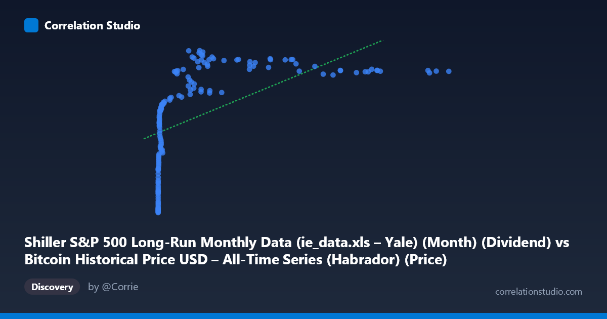
Shiller S&P 500 Long-Run Monthly Data (ie_data.xls – Yale) (Month) (Dividend) vs Bitcoin Historical Price USD – All-Time Series (Habrador) (Price)
- Pearson correlation (r)
- 0.564
- Spearman correlation
- 0.9034
- p-value
- 0
- Sample size (n)
- 155
- 95% confidence interval
- 0.446 to 0.6628
- Granger causality
- None
- Granger optimal lag
- 1
- Time coverage
- 2010-08-01 to 2023-06-01
- Recomputed on refreshed data
- 2026-10-10 (r was 0.564)
AI analysis
Analysis: Bitcoin Price vs. Dividend Data Relationship
1. What the Visualization Reveals
The scatterplot shows a clear non-linear, logarithmic-shaped relationship between the x-variable (mislabeled in the axis metadata, but representing values ranging from near-zero to ~61,374) and Y (ranging 31–71). At low X values (under ~100), Y climbs steeply — from ~31 to ~50 — with small absolute changes in X producing large jumps in Y. Beyond X ≈ 1,000–2,000, the curve flattens considerably, with Y plateauing in the 60–71 range even as X increases by an order of magnitude (from ~10,000 to ~60,000). This classic concave/logarithmic curvature explains why a straight-line fit only captures part of the story.
2. Strength, Direction, and Uncertainty
The Pearson correlation (r = 0.564, r² = 0.318) indicates a moderate positive linear relationship, but only explains ~32% of the variance in Y — meaning roughly two-thirds of Y's variability is driven by other factors or by the nonlinear component of this same relationship. The 95% CI [0.446, 0.663] is reasonably tight and excludes zero, and the p-value (2.13E-14) confirms this correlation is highly statistically significant — not a chance artifact, despite the modest effect size. Critically, the Granger causality tests show no significant predictive direction in either direction (X→Y p=0.486; Y→X p=0.830). This means neither series reliably "leads" the other in time — the correlation appears contemporaneous/structural rather than causal-predictive, which is important since Spearman's ρ exceeding Pearson's r reinforces that the true relationship is stronger than r² suggests, just not linear.
3. Notable Patterns and Features
- Early steep growth zone: Data points with X < 50 show Y sharply rising (31→46), suggesting a log-like or saturating function. - Compression/plateau at high X: From X ≈ 8,000 to 61,000, Y hovers in a narrow 60–71 band, indicating diminishing marginal returns — large X increases yield minimal Y gains. - Mid-range volatility: Around X = 10,000–13,000, Y dips unusually low (60.76–61.33) — an interesting local outlier cluster amid otherwise-high neighboring values (68–70), possibly corresponding to a specific time period or regime shift. - No extreme outliers — the relationship, while noisy, stays within a consistent envelope once log-transformed.
4. Confounding Factors and Caveats
Given the dataset descriptions, this pairing looks like a mismatched or misaligned join — X is labeled as Shiller S&P 500 dividend data but its range (0.06 to 61,374) and scale strongly resemble Bitcoin price history, while Y (31–71) resembles neither raw Bitcoin prices nor typical dividend figures. This suggests column mislabeling or an accidental cross-dataset merge, meaning the "correlation" may be a statistical artifact of two unrelated time series that both trend upward over the 2010–2023 window (a classic spurious correlation via shared time trend). Both Bitcoin and equity-market metrics have grown historically, so co-trending alone could produce this r without genuine economic linkage. Additionally, monthly aggregation and potential differences in sampling frequency/timing between crypto and equity data could introduce alignment errors.
5. Recommendations for Further Investigation
1. Verify data provenance/column mapping — confirm X and Y aren't swapped or mismatched between datasets before drawing economic conclusions. 2. Detrend both series (e.g., using year-over-year returns instead of levels) to test whether the correlation persists after removing shared temporal drift — this is essential given the Granger non-causality result. 3. Fit a log-linear or polynomial model (e.g., Y ~ log(X)) given the Spearman/Pearson discrepancy — this should substantially improve explained variance over the current 31.8%. 4. Segment the analysis by time period to check whether the relationship is stable or driven by specific bull/bear cycles (e.g., 2017, 2020–2021 crypto booms).
X dataset: Bitcoin Historical Price USD – All-Time Series (Habrador)
Y dataset: Shiller S&P 500 Long-Run Monthly Data (ie_data.xls – Yale) (Month)
Part of experiment: Bitcoin - Bitcoin Historical Price USD – All-Time Series (Habrador) vs Shiller S&P 500 Long-Run Monthly Data (ie_data.xls – Yale) (Month)