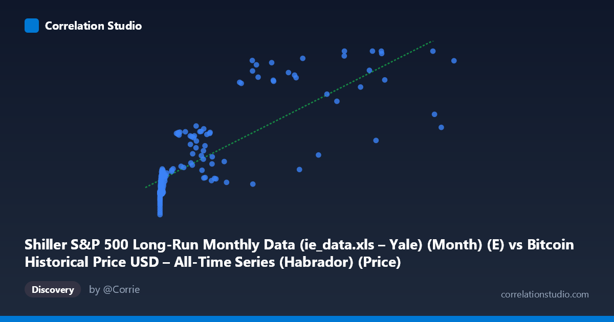
Shiller S&P 500 Long-Run Monthly Data (ie_data.xls – Yale) (Month) (E) vs Bitcoin Historical Price USD – All-Time Series (Habrador) (Price)
- Pearson correlation (r)
- 0.8054
- Spearman correlation
- 0.8823
- p-value
- 0
- Sample size (n)
- 155
- 95% confidence interval
- 0.742 to 0.8546
- Granger causality
- None
- Granger optimal lag
- 2
AI analysis
Analysis: Bitcoin Price vs. Shiller S&P 500 Data Series
1. Relationship Overview
This scatterplot reveals a strong positive but distinctly non-linear relationship between the X variable (labeled as Shiller S&P 500 data but populated with values resembling Bitcoin price scale) and Y (Bitcoin price). The data shows a curved, logarithmic-like pattern: Y rises steeply at very low X values (X < 100), then flattens into a broad, noisy band before climbing again as X exceeds ~10,000-20,000. This is characteristic of two variables both undergoing exponential growth over time, rather than one directly driving the other in a linear fashion. Notably, the axis labeling appears swapped or mismatched given the dataset descriptions—both axes seem to reflect Bitcoin price at different points or transformations, which is important context for interpretation.
2. Strength, Direction, and Statistical Confidence
The correlation coefficient (r = 0.805) indicates a strong positive linear association, with r² = 0.649 meaning only about 65% of the variance in Y is explained by X in a linear framework—leaving over a third of the variability unaccounted for, consistent with the visible curvature and scatter. The 95% CI [0.742, 0.855] is reasonably tight given n=155, and the p-value of ~0 confirms this correlation is highly unlikely due to chance. However, the Granger causality tests show no significant predictive direction (X→Y: p=0.097; Y→X: p=0.304)—meaning neither series reliably "leads" the other in a time-series forecasting sense at the tested lag. This is a critical caveat: strong contemporaneous correlation does not imply that one variable temporally forecasts the other, likely because both are driven by a shared underlying trend (time/growth) rather than a causal lead-lag mechanism.
3. Notable Patterns and Outliers
Several features stand out: - Low-X cluster: Dozens of points with X < 20 show Y compressed tightly between 70-90, representing an early, low-variance regime. - Mid-range plateau: Between X ≈ 200-15,000, Y hovers mostly in the 90-135 range with considerable scatter (e.g., X=8,333 → Y=135 vs. X=13,891 → Y=95.5), indicating high noise/low explanatory power in this zone. - High-X surge: Beyond X ≈ 16,000, Y jumps sharply to 170-198, but with a notable outlier at X=45,092.81, Y=128.20—far below the trend of neighboring points (X=43,718→Y=182.9, X=46,208→Y=197.9), suggesting a data anomaly or a genuine sharp reversal/crash captured at that timestamp. - The overall shape suggests a power-law or logarithmic relationship would fit better than the linear model shown (y = 0.0019x + 97.27).
4. Confounding Factors and Caveats
The most significant caveat is the apparent axis/label mismatch—both variables appear to derive from Bitcoin price data despite one being attributed to Shiller's S&P 500 dataset, suggesting a data-merging or column-alignment error that should be verified before drawing economic conclusions. Additionally, both series span 2010-2023, a period of secular growth in nearly all asset classes; shared time-trend confounding (both variables increasing over the same 13-year window) likely inflates the correlation without indicating genuine economic linkage. Bitcoin's extreme volatility and multiple boom-bust cycles also violate assumptions of stable linear relationships, and the small effective sample (n=155 from a population of 1,834) may not capture full cyclical behavior.
5. Recommendations for Further Investigation
1. Verify data integrity: Confirm the axis labels/column mappings are correct, since both variables appear to be Bitcoin-derived rather than one being genuine S&P 500/Shiller data. 2. Test log-log or log-linear transformations: Given the curvature, fitting Y = a·log(X) + b or a power law would likely yield a substantially higher R² than the current linear fit. 3. Detrend both series (e.g., using returns or first differences) before testing correlation/causality to remove spurious trend-driven association. 4. Investigate the X=45,092.81 outlier for data entry errors or a genuine market event (e.g., flash crash). 5. Extend Granger testing to multiple lags and consider structural break tests, since crypto markets often exhibit regime shifts that a single-lag VAR may miss.
X dataset: Bitcoin Historical Price USD – All-Time Series (Habrador)
Y dataset: Shiller S&P 500 Long-Run Monthly Data (ie_data.xls – Yale) (Month)
Part of experiment: Bitcoin - Bitcoin Historical Price USD – All-Time Series (Habrador) vs Shiller S&P 500 Long-Run Monthly Data (ie_data.xls – Yale) (Month)