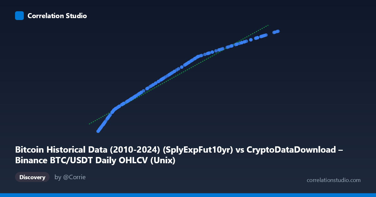
Bitcoin Historical Data (2010-2024) (SplyExpFut10yr) vs CryptoDataDownload – Binance BTC/USDT Daily OHLCV (Unix)
- Pearson correlation (r)
- 0.9833
- Spearman correlation
- 1
- p-value
- 0
- Sample size (n)
- 180
- 95% confidence interval
- 0.9777 to 0.9875
- Granger causality
- None
- Granger optimal lag
- 10
AI analysis
Analysis: Bitcoin Supply Expected in Future (10yr) vs. Time-Indexed BTC Metric
1. What the Visualization Reveals
The scatterplot displays a near-perfect monotonic relationship between the X variable (labeled as a Bitcoin supply-related metric, "SplyExpFut10yr") and the Y variable (a Unix-timestamp-indexed BTC data column) across 180 sampled points spanning August 2017 to February 2026. The data forms a tight, smoothly ascending curve with virtually no scatter around the trend line—points cluster closely along a line with slope ≈2.31×10⁻⁶ and intercept ≈1.68×10⁷. This is characteristic of two variables that both increase steadily and predictably over the observation window.
2. Strength, Direction, and Statistical Confidence
The correlation is extremely strong and positive (r = 0.9833), with r² = 0.9669 indicating that 96.7% of the variance in Y is explained by X (or vice versa, given the linear symmetry). The 95% confidence interval [0.9777, 0.9875] is narrow, and the p-value is effectively zero, meaning the relationship is highly unlikely to be due to chance. However, the Granger causality tests show no significant predictive direction in either direction (X→Y: p=0.097; Y→X: p=0.269, at 10-period lag). This is a critical caveat: despite the near-perfect correlation, neither variable temporally leads the other in a statistically detectable way. This pattern is the classic signature of two variables that are both driven by a shared underlying trend—most likely time itself—rather than one causing the other.
3. Notable Patterns and Features
The relationship appears highly linear at the macro level, but closer inspection of the sample values suggests subtle non-linearity: growth appears slightly front-loaded (steeper early gains from 2017–2019) with some flattening in rate of change toward 2024–2026, though this is minor. No clear outliers or clusters deviate from the main trend—the data is remarkably smooth, consistent with a metric like cumulative/expected supply that changes deterministically (e.g., following Bitcoin's known halving-based emission schedule) rather than a volatile market variable like price. There's no evidence of regime shifts, structural breaks, or bimodal clustering.
4. Confounding Factors and Caveats
The dominant confound here is time as a common driver. Both X (described as "SplyExpFut10yr" — an expected future supply metric) and Y (a timestamp-derived column) are monotonic functions of time, which mechanically produces high correlation without implying any economic or causal linkage. Given that X itself appears to encode a supply schedule (deterministic by protocol design, not market behavior) and Y is described ambiguously as a "Unix" column from an OHLCV dataset, there's a strong possibility this is comparing two derived time-based series rather than genuinely independent economic variables. The lack of Granger causality reinforces that this is likely a spurious or trivial correlation driven by shared temporal trending rather than a meaningful predictive relationship.
5. Actionable Insights
Given the ambiguous column labeling and the trivial time-covariation, the first step should be to verify what X and Y actually represent—if both are essentially transformations of the timestamp/date (e.g., cumulative supply and elapsed time), the high r² is an artifact, not a discovery. Analysts should de-trend both series (e.g., using differencing or detrended residuals) and re-run correlation/Granger tests on the residuals to check for genuine relationships beyond the shared trend. If X truly represents Bitcoin's expected future supply (a known, deterministic emission curve), it should not be used as a predictive feature for market-based Y variables like price or volume without accounting for this deterministic confound. Future work should compare X against genuinely independent market variables (e.g., realized cap growth, active addresses) using detrended or first-differenced data to isolate meaningful signal from mechanical time-trend overlap.
X dataset: CryptoDataDownload – Binance BTC/USDT Daily OHLCV
Y dataset: Bitcoin Historical Data (2010-2024)
Part of experiment: Bitcoin - CryptoDataDownload – Binance BTC/USDT Daily OHLCV vs Bitcoin Historical Data (2010-2024)