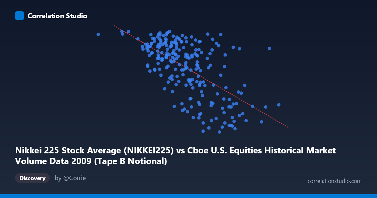
Nikkei 225 Stock Average (NIKKEI225) vs Cboe U.S. Equities Historical Market Volume Data 2009 (Tape B Notional)
- Pearson correlation (r)
- -0.6214
- Spearman correlation
- -0.5852
- p-value
- 0
- Sample size (n)
- 235
- 95% confidence interval
- -0.6942 to -0.536
- Granger causality
- None
- Granger optimal lag
- 10
AI analysis
Analysis: Nikkei 225 vs. Cboe Tape B Notional Volume (2009)
Relationship Overview The scatterplot reveals a moderate negative relationship between the Nikkei 225 daily closing prices and Cboe Tape B notional trading volume in U.S. equity markets throughout 2009. The linear regression equation (y = -4.59×10⁻⁷x + 11,783.1) confirms that as Nikkei 225 values increase, Tape B notional volume tends to decrease. This inverse relationship is visually apparent in the downward-sloping point cloud, with higher Nikkei values (roughly above 7.0 billion on the x-axis) clustering at lower Y values (7,000–8,500), while lower Nikkei values concentrate at higher notional volumes (9,500–10,600). This pattern spans the full year of 2009, a period of significant market recovery following the 2008 financial crisis.
Correlation Strength and Statistical Reliability The Pearson correlation of r = -0.621 indicates a moderate-to-strong negative association, with r² = 0.386 meaning that approximately 38.6% of the variance in Tape B notional volume is statistically explained by Nikkei 225 levels. While meaningful, this also implies that roughly 61.4% of variance remains unexplained, suggesting substantial influence from other factors. The 95% confidence interval of [-0.694, -0.536] is relatively tight and does not cross zero, and the p-value of effectively 0 across a sample of n=235 (drawn from N=3,232) confirms the correlation is highly statistically significant and unlikely to be a chance artifact. However, the Granger causality results are notably non-significant in both directions — Nikkei→Tape B (F=1.018, p=0.429) and Tape B→Nikkei (F=1.297, p=0.234) — meaning that despite the strong contemporaneous correlation, neither variable demonstrates meaningful temporal predictive power over the other at the optimal 10-period lag. The relationship appears to be coincident rather than directionally causal.
Patterns, Clusters, and Outliers The data exhibits a broad but structured scatter with a few identifiable features. There is a visible upper-left cluster where Nikkei values fall below ~4.5 billion and Tape B notional exceeds 10,000, particularly dense between 3.3–4.5 billion on the x-axis. Conversely, a lower-right cluster emerges for Nikkei values above ~6.5 billion, where notional volumes compress into the 7,000–8,800 range. Several potential outliers are noteworthy: the point near (4,440B, 10,581) and (4,120B, 10,585) represent high-volume, low-Nikkei extremes, while (7,069B, 7,376) and (7,346B, 7,280) sit at the low-volume, high-Nikkei extreme. The spread of Y values at mid-range X values (4.5–6.0 billion) is notably wide, suggesting the linear model fits poorly in this central region and that a non-linear or regime-based model might better capture the underlying dynamics.
Confounding Factors and Interpretive Caveats This correlation should be interpreted with considerable caution. 2009 was a structurally unique year — global markets were recovering from the worst financial crisis in decades, with both Japanese equities and U.S. trading volumes heavily influenced by macroeconomic stimulus, risk sentiment shifts, and flight-to-safety dynamics that drove both variables simultaneously rather than causally. The axes appear to have been swapped from their natural intuition (Nikkei is on the X-axis, Tape B notional on Y), which is worth noting when framing interpretation. The correlation likely reflects a common driver — global risk appetite — rather than any direct operational link between Japanese stock prices and U.S. Tape B exchange volume. Seasonality, the timing of specific policy interventions (e.g., TARP, Fed actions), and cross-market contagion could all be confounders. Additionally, Tape B specifically covers NYSE American and regional exchange stocks, a subset of U.S. equity volume, which may behave differently from broader market measures.
Actionable Insights and Further Investigation Given the strong contemporaneous correlation but absent Granger causality, the most productive next step would be to introduce a common proxy for global risk sentiment (e.g., VIX, credit spreads, or TED spread) as a mediating variable to test whether the Nikkei–Tape B relationship persists after controlling for shared macro drivers. A rolling correlation analysis across the 2009 timeline could reveal whether the relationship strengthened during crisis periods (Q1) versus recovery (Q3–Q4), helping identify regime-specific dynamics. Comparing Tape B specifically against Tape A and Tape C notional volumes would clarify whether this pattern is unique to regional exchanges or a broader U.S. market phenomenon. Finally, extending the dataset beyond 2009 into 2010–2011 would test whether this inverse relationship is a crisis-era artifact or a more durable structural feature of the Nikkei–U.S. volume relationship.
X dataset: Cboe U.S. Equities Historical Market Volume Data 2009
Y dataset: Nikkei 225 Stock Average
Part of experiment: Daily - Cboe U.S. Equities Historical Market Volume Data 2009 vs Nikkei 225 Stock Average