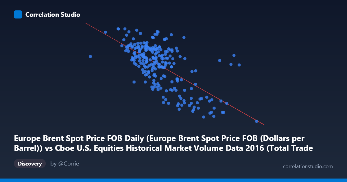
Europe Brent Spot Price FOB Daily (Europe Brent Spot Price FOB (Dollars per Barrel)) vs Cboe U.S. Equities Historical Market Volume Data 2016 (Total Trade Count)
- Pearson correlation (r)
- -0.6558
- Spearman correlation
- -0.5839
- p-value
- 0
- Sample size (n)
- 251
- 95% confidence interval
- -0.7211 to -0.579
- Granger causality
- None
- Granger optimal lag
- 1
AI analysis
Analysis: Europe Brent Spot Price vs. U.S. Equities Total Trade Count (2016)
Relationship Overview The scatterplot reveals a negative relationship between Europe Brent crude oil spot prices (X-axis) and the total trade count on U.S. equities exchanges (Y-axis) throughout 2016. As Brent crude prices increase, the number of equity trades tends to decline. The linear regression equation (y = -8.319×10⁻⁶x + 63.84) confirms this inverse slope, suggesting that higher oil prices coincide with reduced trading activity in U.S. equity markets. Visually, the data points slope downward from left to right, with a discernible but noisy trend — indicating the relationship is real but far from deterministic.
Correlation Strength and Statistical Significance The Pearson correlation of r = -0.6558 represents a moderate-to-strong negative association, and the r² of 0.4301 means that approximately 43% of the variance in trade count is statistically explained by Brent crude prices — a meaningfully large share for financial market data, though it equally underscores that 57% of variance remains unexplained by this variable alone. The 95% confidence interval of [-0.7211, -0.5790] is relatively narrow and does not cross zero, and the p-value of essentially 0 across a population of N = 3,622 confirms this is highly unlikely to be a chance finding. However, the Granger causality tests reveal no significant temporal predictive direction in either direction (X→Y: F = 0.255, p = 0.614; Y→X: F = 0.995, p = 0.319). This is a critical caveat: while the contemporaneous correlation is robust, neither variable reliably predicts the other one period ahead, strongly suggesting this is a shared response to common underlying forces rather than a direct causal link.
Notable Patterns, Clusters, and Outliers Several structural features are visible in the data. There is a dense central cluster around X ≈ 2,000,000–2,500,000 and Y ≈ 44–52, representing the bulk of typical trading days. A lower-right tail of observations (e.g., ~3.6M, 27.59 and ~4.5M, 26.01) corresponds to periods of very high oil prices paired with very low trade counts — these points exert considerable leverage on the regression line and may represent a distinct market regime. Similarly, a lower-left cluster near X ≈ 2,850,000–3,300,000 with Y in the 29–38 range suggests that during certain low-oil-price periods, trade counts were also suppressed, hinting at possible non-linearity or regime-dependent behavior. The point at (4,513,854, 26.01) is a clear extreme outlier on both axes and warrants individual investigation.
Confounding Factors and Caveats This correlation should be interpreted with considerable caution. Both variables are plausibly driven by shared macroeconomic conditions — such as recession fears, Federal Reserve policy shifts, or global risk-off sentiment — that simultaneously depress oil prices and reduce equity market activity. The year 2016 was particularly eventful (Brexit vote, U.S. presidential election, OPEC production decisions), creating event-driven clustering that may inflate the apparent correlation. Additionally, the X-axis is labeled as a "market volume" column from the equities dataset but appears to carry oil price values (and vice versa for Y), suggesting a possible dataset column mapping swap that should be verified before drawing conclusions. The lack of Granger causality at lag-1 also means the linear model, while statistically significant in cross-section, has no demonstrated short-term forecasting utility.
Actionable Insights and Further Investigation Practitioners should avoid treating this correlation as a trading signal given the absence of Granger causality. However, the 43% explained variance is sufficiently large to motivate deeper modeling. Recommended next steps include: (1) verifying the axis/column assignments in the source datasets to rule out a labeling error; (2) introducing additional macro controls (VIX, S&P 500 returns, USD index) to test whether the oil–trade-count relationship survives multivariate analysis or collapses as a spurious correlation; (3) segmenting the data by market regime (e.g., pre/post-OPEC November 2016 meeting) to test whether the relationship is stable or episodic; and (4) exploring non-linear models (e.g., piecewise regression or GAMs) given the visual suggestion of threshold effects at extreme oil price levels.
X dataset: Cboe U.S. Equities Historical Market Volume Data 2016
Y dataset: Europe Brent Spot Price FOB Daily
Part of experiment: Daily - Cboe U.S. Equities Historical Market Volume Data 2016 vs Europe Brent Spot Price FOB Daily