World Bank CO2 Emissions by Country (DataBank) (Liquid Fuel) vs US Employment and Unemployment (labor_force)
- Pearson correlation (r)
- 0.8849
- Spearman correlation
- 0.8753
- p-value
- 0
- Sample size (n)
- 80
- 95% confidence interval
- 0.8257 to 0.9248
- Granger causality
- None
- Granger optimal lag
- 10
AI analysis
Scatterplot Analysis: US Labor Force vs. CO2 Liquid Fuel Emissions
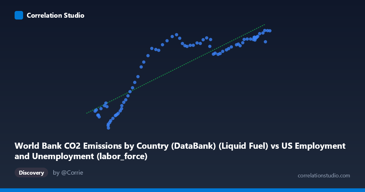
1. Overall Relationship The scatterplot reveals a strong positive association between liquid fuel CO2 emissions and the US labor force size, spanning eight decades of annual observations (1941–2020). As liquid fuel emissions increase, labor force participation rises correspondingly. However, the relationship is notably non-linear: the data traces an elongated S-curve or sigmoid shape, with a steep, scattered lower cluster at low emission values, a transitional mid-range zone, and a compressed upper plateau where labor force values asymptote near 12,000–13,600 units despite continued emission growth. This curvature suggests a linear model, while statistically adequate, is an imperfect structural fit.
2. Correlation Strength and Statistical Framing The Pearson correlation of r = 0.885 indicates a strong positive relationship, and R² = 0.783 means approximately 78.3% of the variance in labor force size is statistically explained by liquid fuel emissions — a substantial share, though ~22% remains unexplained by this variable alone. The 95% confidence interval [0.826, 0.925] is relatively tight and excludes zero entirely, reinforcing reliability across plausible sample variation. The p-value ≈ 0 confirms the correlation is highly unlikely to be a chance artifact at any conventional significance threshold. Critically however, Granger causality is absent in both directions (X→Y: F=1.07, p=0.40; Y→X: F=1.00, p=0.45), meaning neither variable temporally predicts the other beyond baseline trends — this is a co-trending relationship driven by shared time dependency, not a directional causal mechanism.
3. Notable Patterns, Clusters, and Outliers Three distinct visual zones are apparent: - Lower-left cluster (emissions ~53,000–75,000; labor force ~2,500–6,500): High internal scatter relative to the trend, suggesting the early-period relationship was more volatile and less consistent - Mid-range transition zone (~75,000–110,000 emissions): A steep, relatively smooth upward trajectory where the linear model performs best - Upper plateau (~110,000–163,000 emissions): Labor force values compress into a dense band (~11,000–13,600), with emissions continuing to grow — the relationship flattens considerably, violating linear assumptions
A few points warrant individual attention: (62,208; 2,497) and (54,630; 4,556) appear as low-Y outliers in the lower cluster, while (99,008; 12,433) and (104,962; 13,123) sit notably high relative to their X-position in the mid-range, pulling against the plateau trend.
4. Confounding Factors and Caveats The most significant caveat is common time-trend confounding: both variables grew over the 20th century due to macroeconomic expansion, population growth, and industrialization, making spurious correlation nearly inevitable for any two upward-trending US time series over this period. The absence of Granger causality formally confirms this — correlation here reflects parallel historical trajectories, not structural linkage. Additional confounders include: workforce demographic shifts (women entering the labor force post-WWII), energy mix transitions (liquid fuel share declining relative to natural gas and renewables post-1970s), economic recessions (1970s oil shocks, 2008–09, 2020 COVID), and population growth independently driving both variables. The dataset mismatch in labeling (CO2 emissions dataset containing labor force data and vice versa) also warrants verification of the underlying join logic before drawing substantive conclusions.
5. Actionable Insights and Further Investigation - Apply a non-linear model (logarithmic or logistic regression) to better capture the plateau behavior at high emission values; the linear R²=0.783 likely understates fit in the middle range while overstating it at extremes - Detrend both series (e.g., first-differencing or HP filter) before re-assessing correlation to isolate cyclical co-movement from shared secular trend — the Granger null result strongly suggests this is necessary - Segment the analysis by era (pre-1970, 1970–2000, 2000–2020) to test whether the relationship structure changed across energy transition periods and labor market structural shifts - Incorporate per-capita emissions rather than totals to partially control for population growth driving both variables simultaneously - Expand the multivariate framework by adding GDP, population, and energy price indices as controls to isolate any residual direct relationship between fuel consumption patterns and labor market size
X dataset: US Employment and Unemployment
Y dataset: World Bank CO2 Emissions by Country (DataBank)
Part of experiment: Yearly - US Employment and Unemployment vs World Bank CO2 Emissions by Country (DataBank)