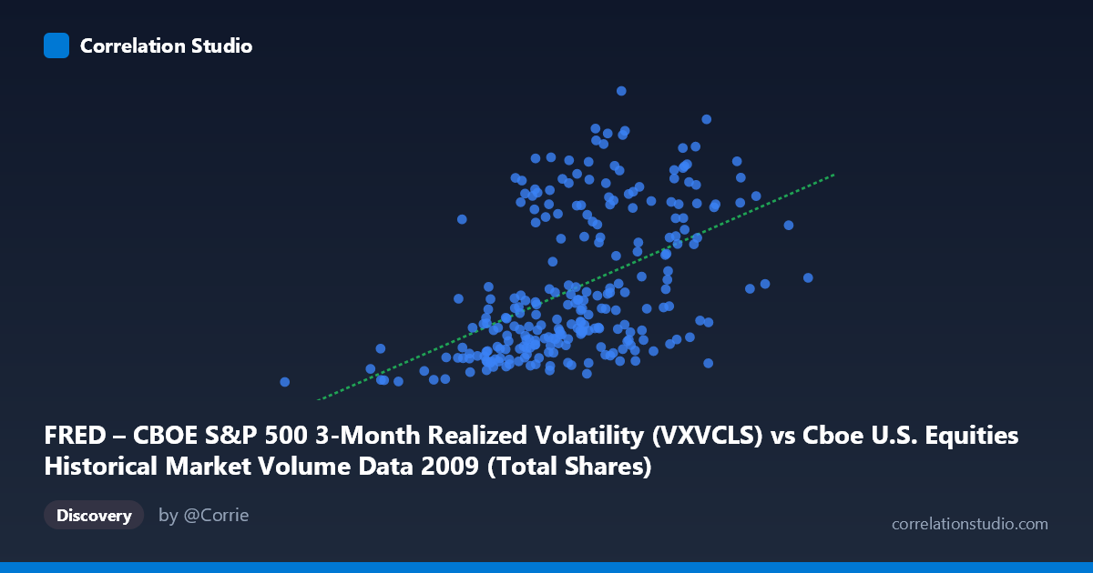
FRED – CBOE S&P 500 3-Month Realized Volatility (VXVCLS) vs Cboe U.S. Equities Historical Market Volume Data 2009 (Total Shares)
- Pearson correlation (r)
- 0.4883
- Spearman correlation
- 0.524
- p-value
- 0
- Sample size (n)
- 252
- 95% confidence interval
- 0.3882 to 0.5771
- Granger causality
- None
- Granger optimal lag
- 1
- Time coverage
- 2009-01-02 to 2009-12-31
- Recomputed on refreshed data
- 2026-10-22 (r was 0.4883)
AI analysis
Scatterplot Analysis: CBOE S&P 500 3-Month Realized Volatility vs. Total Market Shares (2009)
Relationship Overview
The scatterplot reveals a moderate positive relationship between CBOE S&P 500 3-month realized volatility (VXVCLS) and total U.S. equity market shares traded in 2009. As volatility increases, trading volume tends to rise, which aligns with well-established market microstructure theory: elevated uncertainty drives both defensive repositioning and speculative activity, inflating share turnover. The linear regression equation (y = 2.50305E-08x + 13.91) confirms the positive slope, though the wide scatter around the regression line visually signals that this relationship is far from deterministic. The year 2009 is a particularly meaningful context — markets were recovering from the 2008 financial crisis, and the persistence of elevated volatility regimes through much of the year creates natural variation that makes this relationship observable.
Correlation Strength and Statistical Significance
The Pearson correlation of r = 0.4883 indicates a moderate positive association, but the explanatory power is more sobering when framed through R²: only 23.8% of the variance in trading volume is explained by volatility levels, leaving over three-quarters of volume variation unexplained by this single variable. The 95% confidence interval [0.3882, 0.5771] is reasonably tight given the sample size (n = 252), and the p-value of 2.22E-16 confirms the correlation is highly statistically significant — effectively ruling out chance as an explanation. However, statistical significance here is largely a function of the large population (N = 3,232) and adequate sample size rather than indicating a strong practical effect. The Granger causality results are notably non-significant in both directions (X→Y: F = 0.4434, p = 0.506; Y→X: F = 0.3846, p = 0.536), meaning that at a one-period lag, neither variable meaningfully predicts the other temporally. This is an important caveat: the contemporaneous correlation exists, but there is no detectable lead-lag predictive relationship — volatility does not reliably forecast next-period volume, nor vice versa.
Patterns, Clusters, and Outliers
The sample points reveal several noteworthy structural features. There is a visible clustering of observations at lower volatility levels (roughly 22–32 on the Y-axis) paired with a wide range of volume values, suggesting that during calmer periods, volume is highly variable for reasons unrelated to volatility. At higher volatility readings (above ~42–47), there are fewer but more consistently elevated volume observations, hinting at a threshold effect where extreme volatility more reliably drives volume spikes. The point at approximately (192,269,942, 22.43) stands out as a potential low-volume, low-volatility outlier — likely representing an early January trading day or holiday-adjacent session. Similarly, the cluster of high-volatility, high-volume observations (e.g., ~(968M, 46.28), ~(993M, 48.67)) may correspond to specific macro shock events in early 2009. The overall fan-shaped dispersion — where variance in volume appears to increase with volatility — hints at heteroscedasticity, which would violate a key assumption of ordinary least squares regression.
Confounding Factors and Caveats
Several important confounders complicate interpretation. First, the 2009 time period is historically anomalous — the post-crisis recovery introduced structural breaks in both volatility regimes and trading behavior, meaning findings may not generalize to other years. Second, algorithmic and high-frequency trading activity in 2009 was growing rapidly and could inflate share counts independent of volatility sentiment. Third, the axis labels appear swapped relative to convention: the dataset description indicates VXVCLS (volatility) is on the X-axis while total shares are on the Y-axis, but the noted hint suggests the column assignments may be reversed — this warrants verification before drawing causal inferences. Fourth, omitted variables such as index rebalancing days, earnings seasons, Federal Reserve announcements, and options expiration cycles all independently drive both volatility and volume, potentially creating spurious correlation through shared common drivers rather than a direct mechanism.
Actionable Insights and Further Investigation
Practitioners should not use volatility alone as a volume forecasting tool given the weak Granger causality results and modest R² — any trading strategy or liquidity model built solely on this relationship would leave substantial unexplained variance. However, the confirmed positive association does support using volatility as one component of a multi-factor volume prediction model. Further investigation should explore: (1) non-linear or regime-switching models to test whether the volatility-volume relationship strengthens above specific VIX/VXVCLS thresholds; (2) lagged correlations beyond one period to determine if the Granger null holds at longer horizons; (3) controlling for day-of-week, options expiry, and macroeconomic announcement effects to isolate the pure volatility-volume signal; and (4) replicating this analysis across multiple years to assess whether 2009's crisis-recovery dynamics are driving the observed correlation or whether it is structurally persistent.
X dataset: Cboe U.S. Equities Historical Market Volume Data 2009
Y dataset: FRED – CBOE S&P 500 3-Month Realized Volatility
Part of experiment: Daily - Cboe U.S. Equities Historical Market Volume Data 2009 vs FRED – CBOE S&P 500 3-Month Realized Volatility