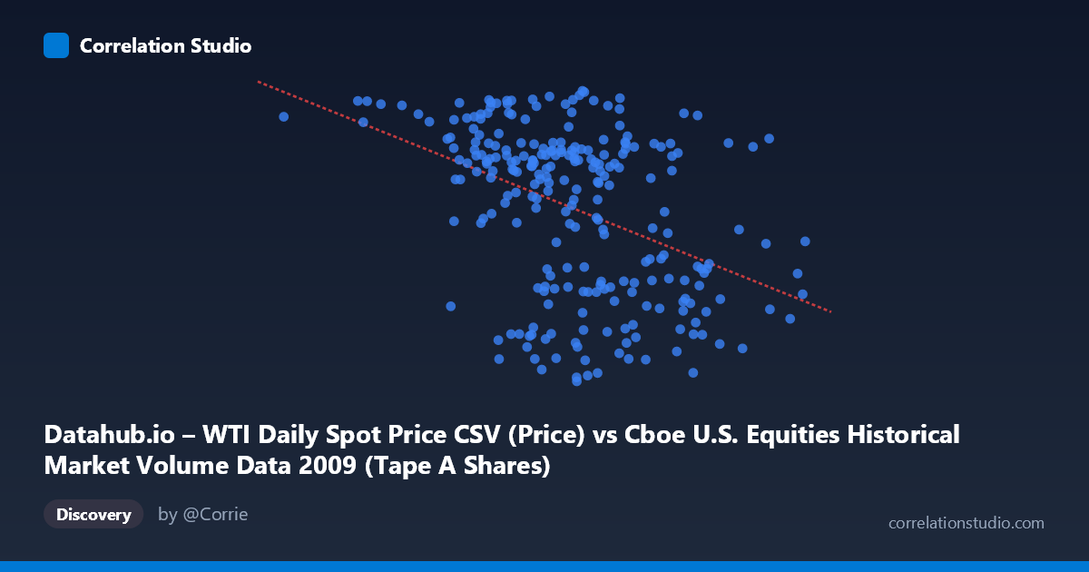
Datahub.io – WTI Daily Spot Price CSV (Price) vs Cboe U.S. Equities Historical Market Volume Data 2009 (Tape A Shares)
- Pearson correlation (r)
- -0.4139
- Spearman correlation
- -0.3987
- p-value
- 0
- Sample size (n)
- 252
- 95% confidence interval
- -0.5114 to -0.306
- Granger causality
- None
- Granger optimal lag
- 1
AI analysis
Analysis: WTI Crude Oil Spot Price vs. Cboe U.S. Equities Tape A Share Volume (2009)
Relationship Overview The scatterplot reveals a moderate negative relationship between U.S. equity market volume (Tape A shares traded) and WTI crude oil spot prices throughout 2009. As equity trading volume increases, oil prices tend to decrease, and vice versa. The linear regression equation (y = -5.66E-08x + 86.82) confirms this inverse slope, suggesting that higher equity market activity is associated with lower crude oil prices. However, the scatter around the regression line is substantial, indicating this relationship is far from deterministic and that many data points deviate considerably from the trend line.
Correlation Strength and Statistical Significance The correlation coefficient of r = -0.414 reflects a moderate negative association. More meaningfully, R² = 0.171, meaning that equity trading volume explains only about 17% of the variance in WTI oil prices — leaving roughly 83% attributable to other factors entirely. While statistically significant (p = 7.49E-12, well below the 0.05 threshold), the 95% confidence interval of [-0.511, -0.306] confirms the true population correlation is reliably negative but modest in magnitude. Critically, the Granger causality tests yield no significant directional predictability in either direction (X→Y: F = 0.47, p = 0.49; Y→X: F = 0.07, p = 0.79). This means that past equity volume does not help predict future oil prices, and past oil prices do not help predict future equity volume — the correlation, though real, carries no demonstrated temporal predictive utility at a one-period lag.
Notable Patterns and Outliers The sample points reveal several noteworthy features. There appears to be a broad spread of Y values (oil prices ranging ~34 to ~81 USD/barrel) across the mid-range of X, suggesting heteroscedasticity — variance in oil prices is not constant across volume levels. A few notable outliers are visible: the point at approximately (105,713,299, 76.83) represents unusually low equity volume paired with high oil prices, consistent with early-2009 crisis conditions when markets were thin but oil had not yet collapsed. Conversely, points clustered around (600–700M shares, 39–45 USD/barrel) suggest periods of heavy trading activity coinciding with depressed oil prices. There is also a visible cluster in the 400–550M share range with a wide spread of oil prices (roughly 37–80 USD/barrel), indicating that moderate trading volume is essentially uninformative about oil price levels.
Confounding Factors and Caveats The 2009 timeframe is critically important context: this was a year of extreme macroeconomic disruption, spanning the tail end of the Global Financial Crisis and a dramatic oil price recovery from late-2008 lows. Both variables were simultaneously driven by broad risk sentiment and economic recovery expectations — a classic confounding factor. When investors fled to safety, equity volumes may have surged amid selling pressure while oil fell; as recovery optimism built, oil rebounded while volumes normalized. This creates a spurious-correlation risk, where the shared influence of macro conditions drives the observed relationship rather than any direct mechanism between trading volume and oil prices. Additionally, the axis labels appear swapped relative to conventional intuition (WTI price is labeled as Y yet described under the X dataset, and vice versa), which warrants verification before drawing firm conclusions.
Actionable Insights and Further Investigation Given the modest explanatory power and absent Granger causality, this correlation should not be used as a predictive trading signal in isolation. However, several avenues merit deeper investigation: (1) Segment the analysis by sub-period within 2009 (Q1 crisis vs. Q3–Q4 recovery) to test whether the correlation structure shifts across market regimes; (2) Introduce a macro risk factor (e.g., VIX, credit spreads) as a control variable to assess whether the X-Y correlation vanishes after accounting for shared risk sentiment; (3) Test non-linear models — the wide scatter at mid-range X values hints that a regime-switching or piecewise model might outperform a simple linear fit; (4) Extend the Granger causality test to multiple lags (2–5 periods) to rule out longer-horizon predictive relationships that a lag-1 test would miss.
X dataset: Cboe U.S. Equities Historical Market Volume Data 2009
Y dataset: Datahub.io – WTI Daily Spot Price CSV
Part of experiment: Daily - Cboe U.S. Equities Historical Market Volume Data 2009 vs Datahub.io – WTI Daily Spot Price CSV