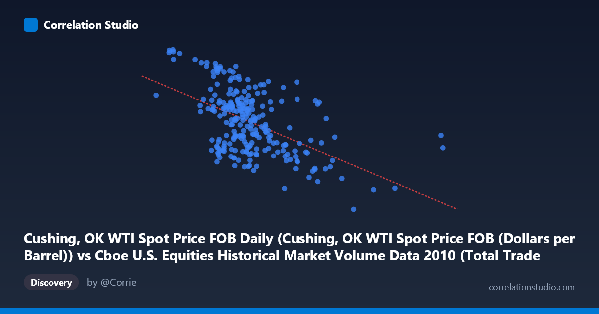
Cushing, OK WTI Spot Price FOB Daily (Cushing, OK WTI Spot Price FOB (Dollars per Barrel)) vs Cboe U.S. Equities Historical Market Volume Data 2010 (Total Trade Count)
- Pearson correlation (r)
- -0.5217
- Spearman correlation
- -0.462
- p-value
- 0
- Sample size (n)
- 252
- 95% confidence interval
- -0.6062 to -0.4256
- Granger causality
- None
- Granger optimal lag
- 1
AI analysis
Analysis: WTI Crude Oil Spot Price vs. Cboe U.S. Equities Total Trade Count (2010)
Relationship Overview
The scatterplot reveals a moderate negative relationship between WTI crude oil spot prices (X-axis) and the total trade count on U.S. equities exchanges (Y-axis) throughout 2010. As oil prices increase, equity trade counts tend to decline — a pattern that is visually apparent across the spread of data points. The linear regression equation (y = -4.17e-06x + 88.79) suggests that for every dollar increase in oil price, trade count decreases by a small but consistent margin. The relationship is not tight — there is considerable vertical scatter at any given X value — but the downward trend is discernible across the range of approximately $64–$91 per barrel.
Correlation Strength, Direction, and Statistical Significance
The Pearson correlation of r = -0.5217 indicates a moderate negative correlation. More meaningfully, R² = 0.2722 tells us that WTI oil prices explain only about 27.2% of the variance in equity trade counts, leaving nearly three-quarters of the variability unexplained by this relationship alone. The 95% confidence interval of [-0.6062, -0.4256] is entirely negative and does not include zero, reinforcing that the negative direction is reliable. With a p-value effectively at zero and a sample of n = 252 drawn from a population of N = 3,302, the correlation is highly statistically significant — the probability of observing this result by chance is negligible. However, statistical significance here reflects the large sample size as much as effect size; the practical magnitude is moderate at best. On Granger causality, neither direction shows significant temporal predictive power at conventional thresholds: X→Y yields F = 0.78, p = 0.38 (clearly insignificant), while Y→X yields F = 3.54, p = 0.061 (marginally suggestive but not significant at the 5% level). This means neither variable reliably predicts future values of the other in a lagged framework, cautioning against any causal interpretation.
Notable Patterns, Clusters, and Outliers
Several features stand out in the sample points. There is a dense cluster in the X range of roughly 1.7M–2.3M (in raw units), corresponding to mid-range trade counts near 75–88, suggesting this is where the bulk of observations fall during typical oil price periods (~$70–$85/barrel). The upper-left region contains high trade counts (85) paired with lower oil prices, consistent with the negative trend. Conversely, high oil price observations (X 3.5M units, e.g., 3,606,177 at Y = 71.88; 4,340,243 at Y = 68.03; 4,002,972 at Y = 64.78) fall noticeably lower on trade count, reinforcing the negative slope. The point at approximately (5,514,533, 75.10) appears as a potential high-leverage outlier — the maximum X value sitting far to the right of the main cluster — which could exert disproportionate influence on the regression line. A few high-Y outliers (e.g., Y ≈ 90.84, 89.83, 89.33) at relatively low X values also merit attention as they represent unusually high trading activity.
Confounding Factors and Interpretive Caveats
The 2010 time period carries significant contextual baggage. Markets were recovering from the 2008–2009 financial crisis, and macroeconomic regime effects — risk sentiment, Federal Reserve policy (quantitative easing), and post-crisis volatility normalization — were all simultaneously influencing both equity trading volumes and commodity prices. Algorithmic and high-frequency trading was expanding rapidly in 2010, which could drive trade count trends independently of oil prices entirely. The correlation may be spurious or driven by a common third factor, such as overall market risk appetite: risk-on periods tend to boost both oil prices and equity activity, while risk-off periods can diverge sharply. Furthermore, the axis labeling appears transposed in the statistical context (X described as trade count in the dataset description but labeled as WTI price in the axis label), which warrants verification of data alignment before drawing firm conclusions. The lack of Granger causality further undermines any directional economic story.
Actionable Insights and Further Investigation
Given that only 27.2% of variance is explained, multivariate modeling is strongly warranted — incorporating variables such as the VIX (equity volatility index), S&P 500 returns, USD index, and macroeconomic indicators would likely capture far more of the trade count variance. Researchers should test for structural breaks within 2010 (e.g., the Flash Crash of May 6, 2010) which could be inflating or distorting the correlation across subperiods. A rolling-window correlation analysis would reveal whether the negative relationship is stable across months or concentrated in specific episodes. The marginal Granger result (Y→X, p = 0.061) — suggesting trade count may weakly predict oil prices — is worth investigating with longer lags or nonlinear Granger frameworks. Finally, removing or separately analyzing the high-leverage outlier at the extreme right of the X distribution would clarify how robust the -0.52 correlation is to that single influential observation.
X dataset: Cboe U.S. Equities Historical Market Volume Data 2010
Y dataset: Cushing, OK WTI Spot Price FOB Daily
Part of experiment: Daily - Cboe U.S. Equities Historical Market Volume Data 2010 vs Cushing, OK WTI Spot Price FOB Daily