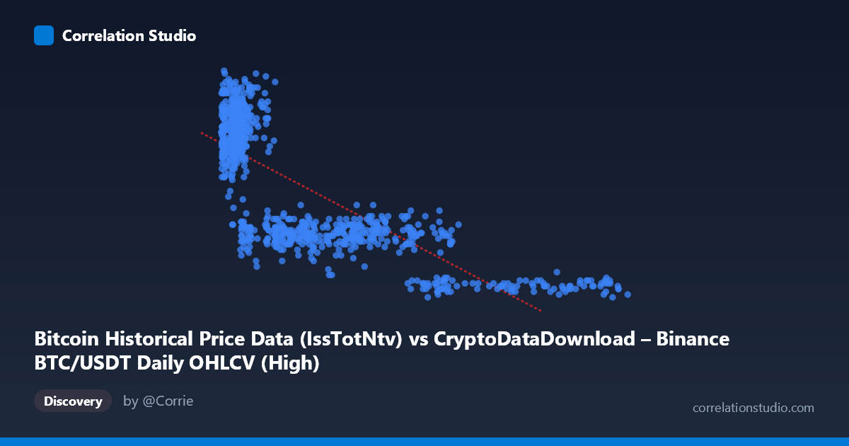
Bitcoin Historical Price Data (IssTotNtv) vs CryptoDataDownload – Binance BTC/USDT Daily OHLCV (High)
- Pearson correlation (r)
- -0.7763
- Spearman correlation
- -0.7599
- p-value
- 0
- Sample size (n)
- 938
- 95% confidence interval
- -0.8005 to -0.7496
- Granger causality
- None
- Granger optimal lag
- 10
- Time coverage
- 2017-08-20 to 2026-05-20
AI analysis
Scatterplot Analysis: BTC/USDT Price Metrics
1. What the Visualization Reveals
The scatterplot shows a clear inverse, curvilinear relationship between the X variable (labeled here as "Bitcoin Historical Price Data," likely a supply/issuance metric given its scale of 3,335–123,763) and Y (the daily High price, ranging $350–$2,375). Rather than a uniform linear decay, the data forms a characteristic hyperbolic/power-law shape: a dense cluster of high-Y, low-X points (X < 15,000, Y 1,600) that curves steeply downward and flattens into a long, thin tail of low-Y, high-X points extending out past X = 100,000.
2. Strength, Direction, and Statistical Confidence
The Pearson correlation of r = -0.7763 indicates a strong negative linear association, with r² = 0.6027 meaning the linear fit explains about 60% of the variance in Y — a substantial but incomplete share, leaving 40% attributable to other factors, nonlinearity, or noise. The tight 95% CI [-0.8005, -0.7496] and p-value of essentially 0 confirm this relationship is highly unlikely to be due to chance, even though n = 938 is a subsample of a larger N = 3,212 population. However, the Granger causality test is the critical caveat: neither direction shows significant predictive power (X→Y: p = 0.33; Y→X: p = 0.74) even at an optimal lag of 10 periods. This means despite the strong contemporaneous correlation, neither variable temporally "leads" the other — the relationship is likely structural/mechanical (e.g., both derived from the same underlying price series) rather than a causal, forecastable dynamic over time.
3. Notable Patterns and Outliers
The shape strongly suggests a non-linear, inverse (1/x-like) relationship rather than a truly linear one — the data hugs a curve that a straight line only approximates. Two regimes are visible: a "high-price era" cluster (X roughly 3,000–15,000, Y = 1,600–2,375) and a "low-price/mature era" tail (X = 60,000–124,000, Y = 400–950) with much lower variance. Points like (101,899, 425) and (118,452, 500) sit at the extreme tail and exert leverage on the linear fit. Given the metadata, this pattern is consistent with X being a cumulative or growing metric (e.g., total transacted native units, block height proxy, or circulating supply-adjusted value) that mechanically decreases in relation to price highs as the network matures — not two independent market signals.
4. Confounding Factors and Caveats
The most important caveat: X and Y appear to be near-duplicate or derived series from the same underlying dataset (both reference "Binance BTC/USDT Daily OHLCV"). This raises concern about spurious/tautological correlation — if X is a transformation of price or volume tied to the same OHLCV table, the negative relationship may reflect a definitional or accounting relationship rather than an economic one. Additionally, this is time-series data spanning 2017–2026, so autocorrelation within each variable (trending prices, trending supply metrics) can inflate r without indicating genuine bivariate dependence — a classic case where two non-stationary trending series appear correlated. The non-Granger result reinforces that this is likely a contemporaneous/structural artifact, not a dynamic causal link.
5. Recommendations for Further Investigation
1. Clarify variable definitions — confirm exactly what the X-axis metric represents (units, calculation method) to rule out a tautological relationship with Y. 2. Test for non-linearity — fit a power/log or reciprocal model (e.g., Y ~ 1/X or log-log regression) which likely will outperform the current linear R² = 0.60 given the visible curve. 3. Difference or detrend both series before correlating, to check whether the relationship survives after removing shared time trends (a standard fix for spurious time-series correlation). 4. Segment by era (e.g., pre-2020 vs. post-2020) to see if the relationship is stable or driven entirely by structural regime shifts in Bitcoin's market cycle. 5. Given the lack of Granger causality, avoid using this pair for predictive/forecasting models; treat the correlation as descriptive/structural rather than a trading or causal signal.
X dataset: CryptoDataDownload – Binance BTC/USDT Daily OHLCV
Y dataset: Bitcoin Historical Price Data
Part of experiment: Bitcoin - CryptoDataDownload – Binance BTC/USDT Daily OHLCV vs Bitcoin Historical Price Data